
11868 LLM Sys: Distributed Training, DDP, and Model Parallelism
Lec13 Distributed Training
This lecture is about the communication side of large-scale training: why modern LLMs need distributed execution, what collective communication primitives NCCL provides, and why AllReduce-based data parallelism became the standard design.
Why Distributed Training Becomes Necessary
Modern LLMs are trained at a scale that makes single-device training unrealistic:
- DeepSeek-V3 (671B): trained on 2,048 H800 GPUs for about 2 months, totaling 2.664 million H800 GPU hours
- LLaMA 3.1 (405B): trained with 16,000 H100 GPUs, totaling 30.84 million GPU hours
There are two scaling pressures at the same time:
- Model size keeps increasing
- Training data size keeps increasing
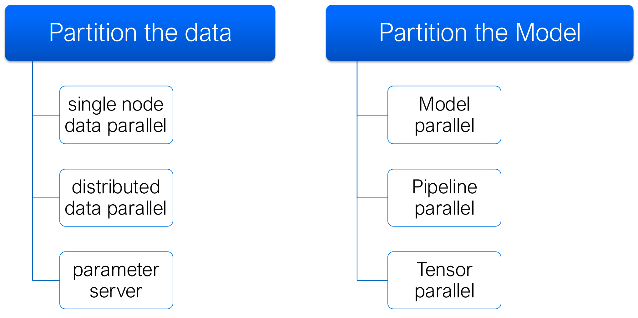
Strategies for Scalable Training
At a high level, large-scale training systems combine one or more of the following strategies:
- Data parallelism: replicate the model, split the data
- Parameter server: centralize parameter updates
- Model / tensor parallelism: split the model itself
- Pipeline parallelism: split layers across devices
Lec13 focuses on the case where the model still fits on each GPU, so the main tool is data parallel training.
Classical Distributed Training: Parameter Server
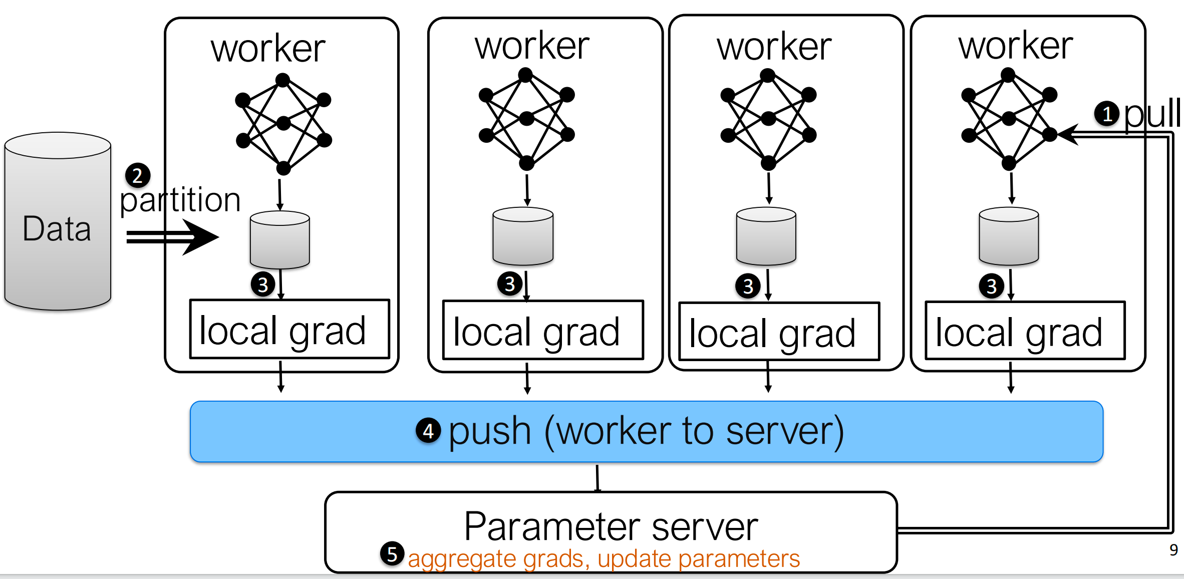
The classical setup is the parameter server architecture:
- Split the mini-batch across workers
- Each worker runs forward and backward locally
- Workers push local gradients to a central server
- The server aggregates gradients and updates parameters
- Workers pull the updated parameters back
This design is conceptually simple, but it has two major problems:
- It introduces a central bottleneck
- It requires two synchronization directions per
iteration:
- gradients go from workers to server
- parameters go from server to workers
In practice, the lecture maps this design to NCCL primitives naturally:
- Pull parameters:
Broadcast - Push gradients:
Reduce
The problem is that the server becomes a traffic hotspot. As the number of workers grows, the server has to absorb and emit more and more data every iteration.
Multi-GPU Communication with NCCL
NCCL (NVIDIA Collective Communication Library), which is the standard communication layer behind many multi-GPU training systems. It provides:
- Collective communication primitives
- Point-to-point send/receive
- Support for different interconnects:
- PCIe
- NVLink
- InfiniBand
- IP sockets
An important systems detail is that NCCL operations are tied to a CUDA stream, so communication can be coordinated with GPU compute and potentially overlapped.
NCCL Primitives
The core primitives from the lecture are:
| Primitive | Meaning |
|---|---|
Broadcast |
copy data from one root rank to all ranks |
Reduce |
aggregate data from all ranks onto one root rank |
AllReduce |
aggregate data and write the result to every rank |
ReduceScatter |
reduce first, then scatter partitions of the result |
AllGather |
gather partitions from all ranks and replicate the full result |
One key identity appears repeatedly:
\[ \text{AllReduce} = \text{ReduceScatter} + \text{AllGather} \]
This decomposition is not just conceptual. It is exactly how efficient ring-based AllReduce is typically implemented.
Why Rings Matter
NCCL uses ring-based communication heavily because a ring avoids a central bottleneck and keeps all links busy.
The lecture uses broadcast to explain the idea. Suppose there are
K ranks, each link has bandwidth B, and the
message size is N.
If we broadcast naively along a unidirectional ring:
\[ T_{\text{ring-broadcast}} = (K-1)\frac{N}{B} \]
That looks bad because the full message must move hop by hop.
But if we split the message into S chunks and
pipeline them through the ring, the total time
becomes:
\[ T_{\text{pipelined}} = (K-2+S)\frac{N}{SB} \]
When S is large enough, this approaches:
\[ T_{\text{pipelined}} \approx \frac{N}{B} \]
The main idea is simple: chunking + pipelining converts a latency-heavy collective into a bandwidth-efficient one.
Grouped Communication
When one process manages multiple GPUs, NCCL often uses:
1 | ncclGroupStart(); |
This lets the runtime batch related communication calls together. The
lecture shows this both for communicator initialization and for
launching multiple ncclAllReduce calls across devices.
Data Parallel Training via AllReduce
The main workflow of data parallel training is:
- Partition the mini-batch across workers
- Each worker runs forward + backward on its local shard
- Workers synchronize gradients
- Every worker performs the same optimizer step
So unlike a parameter server, there is no special update node. Every worker keeps a full model replica, and after gradient synchronization all replicas remain identical.
Why Local Optimizer Updates Are Fine
At first glance, updating parameters on every GPU looks redundant: why not update once and send the new parameters around?
The answer from the lecture is practical:
- Local parameter updates are cheap
- Inter-GPU data transfer is expensive
So it is usually better to synchronize gradients once, then let each worker apply the same update locally.
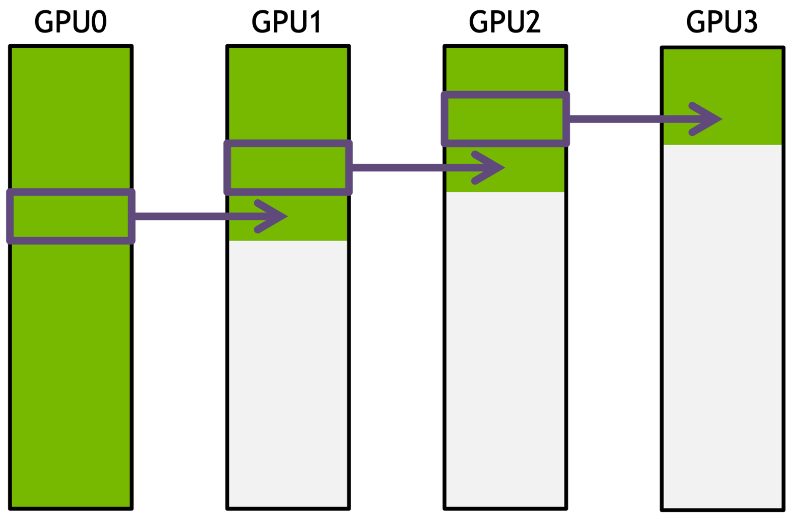
Ring AllReduce
The lecture focuses on Ring AllReduce, which is the standard data-parallel synchronization pattern in systems like NCCL, Horovod, and DDP.
Assume there are K workers and a gradient tensor of
total size M.
Phase 1: Reduce-Scatter
- Split the gradient tensor into
Kchunks - Arrange workers in a logical ring
- In each of the
K-1steps:- each worker sends one chunk to its right neighbor
- each worker receives one chunk from its left neighbor
- the received chunk is accumulated into the local partial result
After K-1 steps, each worker owns one fully
reduced chunk.
Phase 2: AllGather
- Start from the reduced chunks produced above
- Again communicate for
K-1steps around the ring - Each step forwards one completed chunk
At the end, every worker has the full reduced gradient tensor.
Communication Cost
Each step transmits only M / K data per worker. Since
there are 2(K-1) steps in total:
\[ \text{communication per worker} = 2(K-1)\frac{M}{K} \approx 2M \]
This is the key scalability result: the total communication
per worker is roughly constant with respect to
K, while the load is evenly distributed across the
ring.
Simplified Pseudocode
The lecture also shows MPI-style implementations for the two phases.
Reduce-Scatter
1 | for i in 0 .. K-2: |
AllGather
1 | for i in 0 .. K-2: |
The low-level code is less important than the systems idea: reduce while circulating chunks, then circulate the completed chunks.
Parameter Server vs AllReduce
Both approaches synchronize workers, but they do so differently:
| Method | Communication Pattern | Main Limitation |
|---|---|---|
| Parameter Server | workers push grads, server updates, server broadcasts params | central bottleneck |
| AllReduce Data Parallel | workers collaborate directly to aggregate gradients | model still replicated on every worker |
The lecture’s conclusion is straightforward:
- Parameter server is simple but poorly balanced
- AllReduce data parallelism removes the central bottleneck and is the preferred design for synchronous GPU training
Lec13 Takeaways
- Large-scale LLM training is impossible on a single GPU because both model size and data scale have exploded.
- NCCL provides the core collective primitives used in practice for inter-GPU communication.
- Ring-based communication matters because chunking and pipelining use bandwidth much more efficiently than naive collectives.
- Synchronous data parallel training usually prefers AllReduce over a parameter server because it avoids a central bottleneck.
Lec14 Distributed Data Parallel Training
Lec14 moves from communication primitives to framework implementation. The central question is: how can a framework expose distributed data parallel training with minimal code changes while still overlapping communication with backward computation?
From Data Parallelism to DDP
Once the communication pattern is clear, the next question is: how should a framework expose it to users?
PyTorch’s answer is Distributed Data Parallel (DDP).
Conceptually, DDP is still data parallelism:
- each process has a model replica
- each process runs local forward/backward
- gradients are synchronized across all processes
- optimizers run locally but remain identical
The difference is that DDP is an efficient implementation of that idea across multiple nodes and multiple GPUs.
Design Goals of DDP
The lecture highlights two design goals from the PyTorch Distributed paper:
- Non-intrusive: users should be able to reuse a local training script with minimal changes
- Interceptive: the framework should be able to intercept gradient events and trigger communication as early as possible
This second point is the key to DDP’s performance.
Distributed Process Setup
DDP works in terms of distributed processes.
The lecture distinguishes:
- World size: total number of processes
- Global rank: the unique process ID in the whole job
- Local rank: the process ID within one node
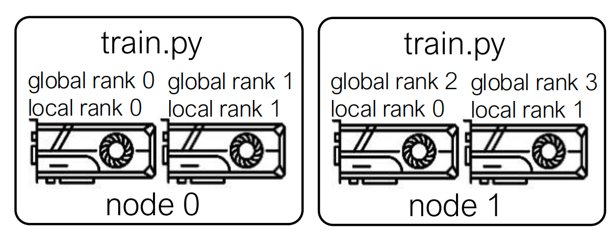
In a multi-node run, each node launches one or more local processes. A launcher passes process-group metadata such as:
MASTER_ADDRMASTER_PORTRANKWORLD_SIZE
Then each process initializes distributed communication:
1 | import argparse |
A Minimal DDP Training Skeleton
The lecture shows a minimal usage pattern:
1 | import torch |
In a real training job, the data loader should also be sharded so different ranks process different examples, but the core idea is unchanged.
Why a Naive DDP Implementation Is Not Enough
A naive implementation would do this:
- Run the entire backward pass
- Wait until all gradients are computed
- Launch one big AllReduce
- Run the optimizer step
This is correct, but inefficient, because it serializes:
- backward computation
- communication
That means GPUs spend part of the iteration waiting for gradients to finish computing, and then another part waiting for communication to finish.
Gradient Bucketing
DDP improves on the naive approach with gradient bucketing.
Instead of waiting for all gradients, DDP:
- Groups parameter gradients into buckets
- Monitors when each gradient becomes ready during backward
- Launches an asynchronous AllReduce as soon as one bucket is complete
This lets communication overlap with the rest of backpropagation.
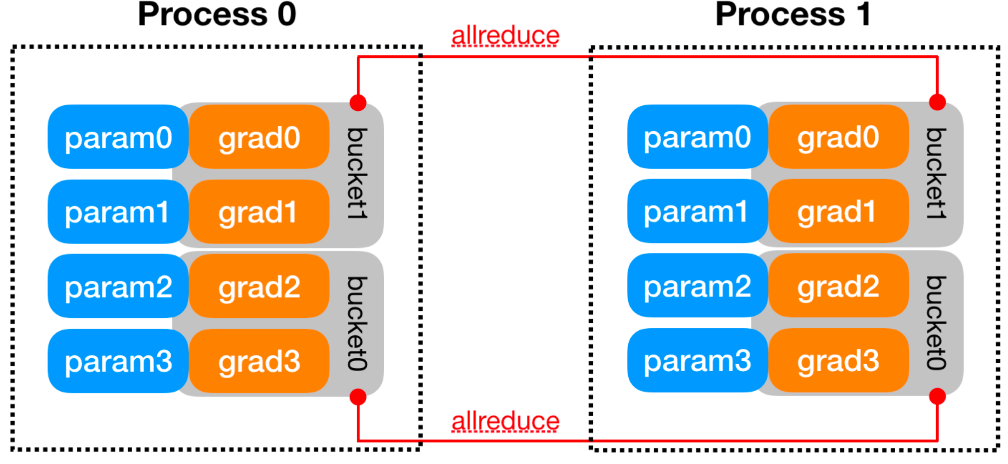
Bucket Construction
The lecture notes several practical details:
- Bucket size is configurable with
bucket_cap_mb - The mapping from parameters to buckets is fixed at construction time
- Parameters are placed into buckets in roughly the reverse
order of
model.parameters()
That reverse ordering is intentional. During backward, gradients usually become ready from the last layer back to the first, so reverse ordering helps entire buckets become ready earlier.
The Tradeoff in Bucket Size
Bucket size is a classic systems tradeoff:
- Small buckets
- more overlap opportunities
- but more collectives and higher latency overhead
- Large buckets
- fewer collective calls
- but less overlap between communication and computation
So DDP is not only about using AllReduce. It is about using AllReduce at the right granularity.
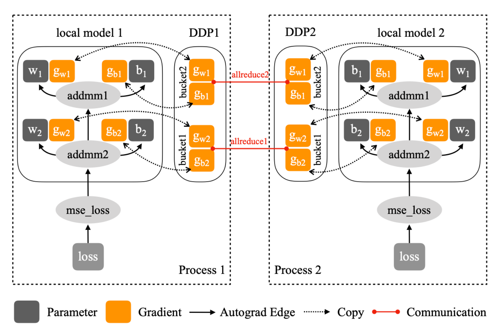
How DDP Intercepts Backward
The reducer in DDP registers an autograd hook for each parameter. When a parameter’s gradient is produced and accumulated, the hook marks that parameter as ready.
A simplified version of the lecture’s logic is:
1 | autograd_hook(param_i): |
The real implementation keeps more metadata, but the key mechanism is:
- each parameter completion triggers a hook
- hooks decrement the bucket’s pending count
- when a bucket reaches zero pending gradients, DDP launches communication immediately
The lecture shows this flow through functions such as:
autograd_hookmark_variable_readymark_bucket_readyall_reduce_bucket
That is the “interceptive” part of DDP’s design.
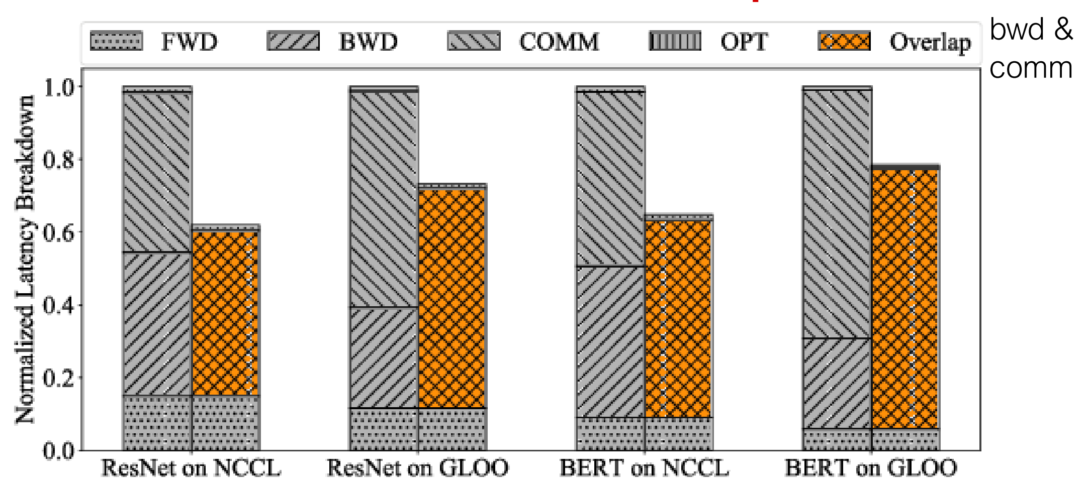
Overlapping Communication with Computation
This is the main performance win of DDP.
During backward:
- upper layers finish first and produce gradients
- DDP launches AllReduce for ready buckets
- deeper parts of backward continue running while earlier buckets are already communicating
So the iteration timeline becomes:
- backward compute
- communication
not as two disjoint blocks, but as partially overlapping work on the GPU and network.
This reduces exposed communication latency and improves scalability.
What DDP Really Optimizes
At a high level, DDP is still just synchronous data parallel training. What it optimizes is the execution schedule:
- it avoids waiting until all gradients are ready
- it batches gradients to avoid excessive communication overhead
- it overlaps collective communication with backward compute
That is why DDP scales much better than the naive “backward first, AllReduce later” design.
Practical Interpretation
The two lectures together suggest a useful way to think about the stack:
- Algorithmic level: use synchronous data parallelism
- Communication level: implement gradient synchronization with efficient collectives like Ring AllReduce
- Framework level: expose the model as ordinary PyTorch code while letting DDP schedule communication automatically
This is also why DDP is widely adopted in practice: it gives most of the benefit of optimized distributed training without requiring users to manually write communication code.
Limits of DDP
DDP solves only one part of the scaling problem.
It works well when:
- the model fits on every GPU
- the main challenge is speeding up training by splitting data across workers
It does not solve the case where the model replica itself is too large for one device. In that setting, one needs more aggressive techniques such as:
- tensor / model parallelism
- pipeline parallelism
- optimizer and parameter sharding methods such as ZeRO or FSDP
So DDP should be viewed as the default solution for scalable synchronous data parallel training, not as the full solution to large-model training.
Lec14 Takeaways
- DDP keeps the data-parallel programming model, but implements it more efficiently than a naive post-backward AllReduce.
- The core optimization is gradient bucketing: synchronize a bucket once all gradients inside it are ready.
- Autograd hooks let DDP intercept backward execution and launch communication early.
- The main systems win is overlapping backward compute with AllReduce communication.
Lec15 Model Parallel Training
Lec15 addresses the setting where a model is too large to fit on a single GPU. The central question is: how can we partition a model’s computation across multiple devices while minimizing idle time and communication overhead?
Why Model Parallelism Is Needed
Model sizes have grown exponentially. A single GPU (e.g., 80GB H100) cannot hold a 175B parameter model even in FP16 — parameters alone would require ~350GB, plus optimizer states and activations. When the model no longer fits on one device, data parallelism is insufficient. Model parallelism splits the model itself across devices to make training feasible.
Two Forms of Model Parallelism
Model parallel training partitions the model’s computation (forward, backward, update) across multiple workers. There are two main approaches:
| Form | What It Splits | Granularity |
|---|---|---|
| Pipeline Parallelism | layers across devices | layer-wise (horizontal) |
| Tensor Parallelism | weight matrices within a layer | tensor-wise (vertical) |
A third form, expert parallelism (for MoE models), is covered in a later lecture.
Pipeline Parallelism
Naive Model Parallelism
The simplest approach assigns different layers to different GPUs:
- Device 0 holds layer 0, device 1 holds layer 1, etc.
- Forward pass flows from device 0 → device 1 → … → device K-1
- Backward pass flows in reverse
- Inter-device communication uses NCCL point-to-point send/recv
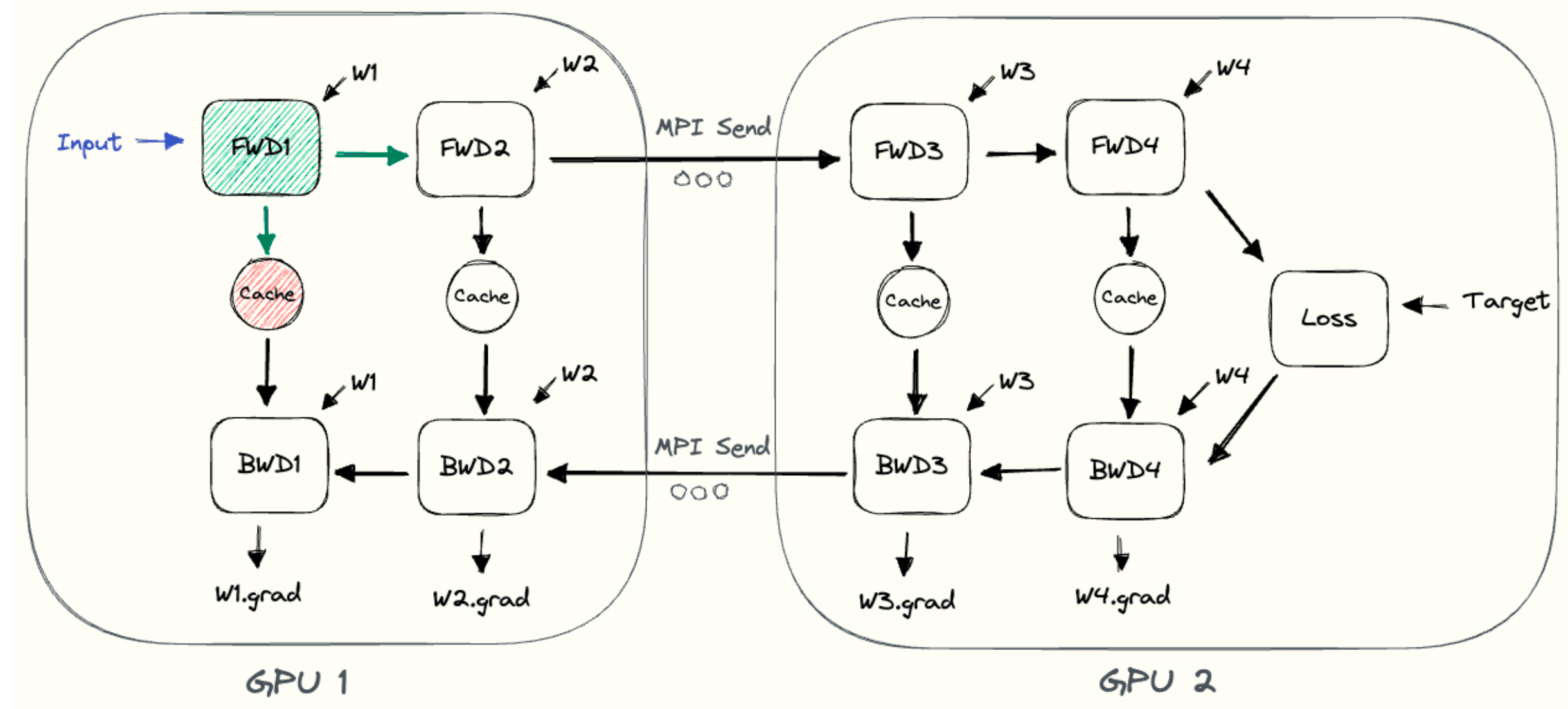
A concrete PyTorch example splits a ResNet50 across two GPUs:
1 | class ModelParallelResNet50(ResNet): |
The .to('cuda:1') call in forward triggers an implicit
NCCL send/recv to move activations between devices.
The critical problem: at any point in time, only one GPU is active. All other GPUs are idle waiting for activations or gradients to arrive.
Limitations of Naive Pipeline Parallelism
- Low GPU utilization: only one device is computing at any moment
- No overlap of computation and communication: while sending intermediate results to the next device, GPUs sit idle
- High memory demand: the first GPU must store all activations until the entire batch completes backward
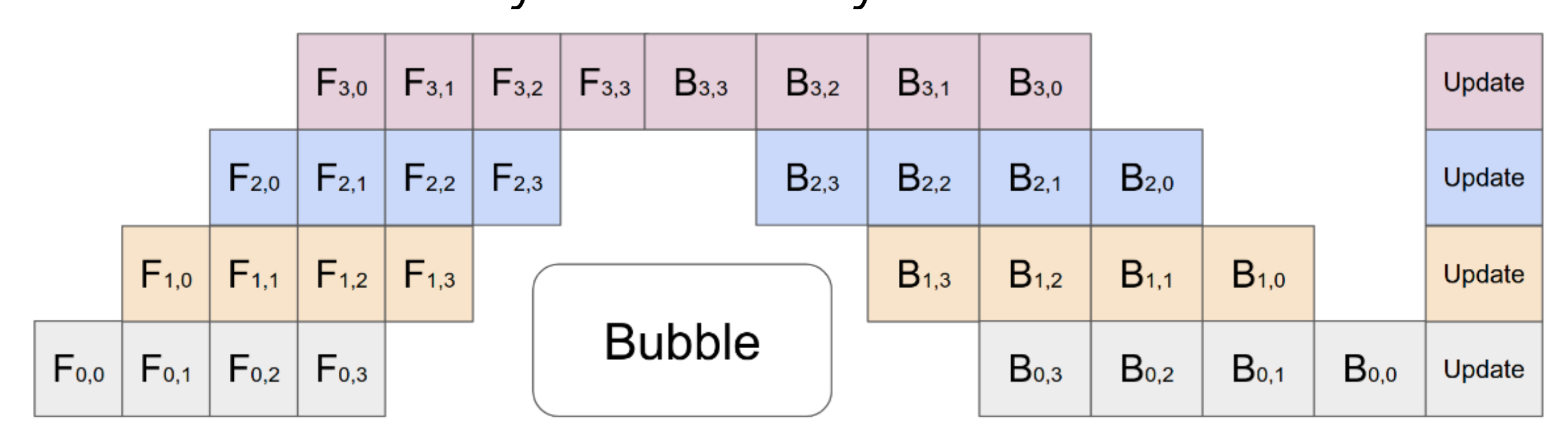
GPipe: Microbatch Pipelining
GPipe (Huang et al., NeurIPS 2019) addresses these problems with a simple but effective idea: split the mini-batch into smaller micro-batches and pipeline them.
The key parameters are:
- \(K\): number of pipeline stages (devices)
- \(M\): number of micro-batches
- \(L\): number of model layers
The workflow:
- Divide the input mini-batch into \(M\) micro-batches
- Each micro-batch’s forward result is sent to the next device immediately once that stage completes
- All forwards complete before any backward begins
- During backward, GPipe recomputes the forward pass for each micro-batch (gradient checkpointing), then sends gradients immediately once ready
This creates a pipeline where multiple GPUs can work simultaneously on different micro-batches.
Bubble overhead:
\[ O\left(\frac{K-1}{M+K-1}\right) \]
This becomes negligible when \(M > 4 \times K\). If you have 4 pipeline stages, using 16 or more micro-batches keeps the bubble small.
Communication overhead: only activation tensors at partition boundaries need to be transferred between adjacent stages.
Peak activation memory: with gradient checkpointing, memory drops from \(O(N \times L)\) to \(O(N + \frac{L}{K} \times \frac{N}{M})\), where \(N\) is the batch size.
GPipe Performance
Normalized training throughput using GPipe with different numbers of partitions \(K\) and micro-batches \(M\):
TPU results:
| \(K =\) | 2 | 4 | 8 | 2 | 4 | 8 |
|---|---|---|---|---|---|---|
| AmoebaNet | Transformer | |||||
| \(M = 1\) | 1 | 1.13 | 1.38 | 1 | 1.07 | 1.3 |
| \(M = 4\) | 1.07 | 1.26 | 1.72 | 1.7 | 3.2 | 4.8 |
| \(M = 32\) | 1.21 | 1.84 | 3.48 | 1.8 | 3.4 | 6.3 |
More micro-batches consistently improve throughput, confirming that pipelining is essential for GPU utilization. The Transformer model benefits more because its layers are more uniform, leading to better load balance across pipeline stages.
Gradient Checkpointing
GPipe uses gradient checkpointing (also called re-materialization) to reduce activation memory during pipeline execution.
The idea explores three points on the memory-computation tradeoff:
| Strategy | Activation Memory | Computation Cost |
|---|---|---|
| Vanilla backprop (store all) | \(O(n)\) | \(O(n)\) |
| Memory-poor (store nothing) | \(O(1)\) | \(O(n^2)\) |
| Gradient checkpoint (store every \(\sqrt{n}\)) | \(O(\sqrt{n})\) | \(O(n)\) |
The practical choice is gradient checkpointing: cache activations at every \(\sqrt{n}\) layers. During backward, recompute only the activations between checkpoints. This achieves sublinear memory with only a modest increase in computation (roughly 33% more forward work).
Limitations of GPipe
GPipe finishes all forward passes before starting any backward. This means all micro-batches that have completed forward but not yet started backward must keep their activations in memory.
In the lecture’s example with 4 devices and 8 micro-batches, the peak number of in-flight micro-batches (completed forward but not backward) is 8. All their activations must be stored simultaneously, which can be a significant memory burden.
PipeDream-Flush: 1F1B Scheduling
PipeDream-Flush (Narayanan et al., SOSP 2019) improves on GPipe by starting backward as soon as possible using a one-forward-one-backward (1F1B) schedule.
Instead of completing all forwards first, after a warmup phase, each device alternates between forward and backward passes on different micro-batches. The benefit is clear:
- Reduced activation memory: the maximum number of in-flight micro-batches drops to at most \(K\) (the number of pipeline stages), compared to \(M\) in GPipe
- In the same 4-device example (assuming 1 backward ≈ 2× the time of 1 forward), the peak in-flight count drops from 8 to 4
The bubble overhead remains similar to GPipe, but the memory savings are substantial.
Interleaved Stages (Megatron-LM)
Megatron-LM (Narayanan et al., SC 2021) further reduces the pipeline bubble by chunking model layers and interleaving stages.
Instead of assigning a contiguous block of layers to each device, each device holds multiple non-contiguous chunks:
| Chunk 1 Layers | Chunk 2 Layers | |
|---|---|---|
| Device 1 | 1, 2 | 9, 10 |
| Device 2 | 3, 4 | 11, 12 |
| Device 3 | 5, 6 | 13, 14 |
| Device 4 | 7, 8 | 15, 16 |
Each chunk computes a smaller piece of work, and the schedule interleaves forward/backward across chunks. This creates more pipeline stages with finer granularity, which reduces the bubble fraction further at the cost of more inter-device communication.
Pipeline Parallelism Implementation
The lecture shows implementation patterns at two levels.
Low-level scheduling (GPipe pattern):
1 | def minibatch_steps(self): |
Each forward step either loads data (first stage) or receives activations from the previous stage via non-blocking communication, runs forward, and sends activations to the next stage.
PyTorch’s torch.distributed.pipelining
provides a higher-level API with two components:
PipelineStage: wraps a model partition for a specific devicePipelineSchedule: orchestrates execution (e.g.,ScheduleGPipe)
The model is designed so that layers can be selectively deleted per stage:
1 | class Transformer(nn.Module): |
Using ModuleDict and guarding with
if self.X else allows each stage to skip components it does
not own. The schedule then handles micro-batching and inter-stage
communication automatically:
1 | from torch.distributed.pipelining import PipelineStage, ScheduleGPipe |
Tensor Parallelism
Tensor parallelism splits individual matrix operations within a single layer across multiple GPUs. Unlike pipeline parallelism which splits across layers, tensor parallelism splits within a layer.
Basic Idea: Splitting Matrix Computation
For a matrix multiplication \(C = A \cdot B\), we can split the weight matrix \(B\) column-wise across GPUs:
\[ B = [B_1, B_2], \quad C_1 = A \cdot B_1, \quad C_2 = A \cdot B_2 \]
Each GPU computes its own partial result. An AllGather then assembles the full output \(C = [C_1, C_2]\) across all GPUs.
Tensor Parallelism for the FFN Block
The Transformer FFN block computes:
\[ Y = \text{GeLU}(X \cdot A), \quad Z = \text{Dropout}(Y \cdot B) \]
A naive split of both \(X\) and \(A\) would require an AllReduce before the GeLU, because GeLU is nonlinear:
\[ \text{GeLU}(X_1 A_1 + X_2 A_2) \neq \text{GeLU}(X_1 A_1) + \text{GeLU}(X_2 A_2) \]
The Megatron-LM solution avoids this by splitting only the weight matrices in a complementary way:
- Split \(A\) column-wise: \(A = [A_1, A_2]\)
- Split \(B\) row-wise: \(B = \begin{bmatrix} B_1 \\ B_2 \end{bmatrix}\)
This gives:
\[ [Y_1, Y_2] = [\text{GeLU}(X \cdot A_1),\; \text{GeLU}(X \cdot A_2)] \]
Each GPU can independently compute its \(Y_i\) — no AllReduce needed for the intermediate result. Then:
\[ Z = Y_1 \cdot B_1 + Y_2 \cdot B_2 \]
This final sum requires an AllReduce to aggregate the partial results across GPUs. The key win is that only one AllReduce per FFN block is needed, not two.
Tensor Parallelism for Self-Attention
Self-attention has a natural parallelism axis: attention heads. The Q, K, V projection matrices are split column-wise by heads:
\[ Q = [Q_1, Q_2], \quad K = [K_1, K_2], \quad V = [V_1, V_2] \]
Each GPU computes attention for its assigned heads independently. Since attention heads are independent computations, no AllReduce is needed for the intermediate result. Only the output projection requires an AllReduce, similar to the FFN block.
The output projection matrix \(B\) is split row-wise (\(B = \begin{bmatrix} B_1 \\ B_2 \end{bmatrix}\)), and the final result is summed across GPUs via AllReduce.
Tensor Parallelism for Embeddings
- Input embedding: split the embedding table column-wise (\(E = [E_1, E_2]\)). An AllReduce is required to combine partial embeddings.
- Output embedding: also split column-wise. The GEMM produces partial logits \([Y_1, Y_2] = [X E_1, X E_2]\). By fusing the cross-entropy loss with the partial logits, the communication cost is hugely reduced — only scalar losses need to be aggregated rather than full logit vectors. An AllGather is needed otherwise.
Components That Are Duplicated
Some operations are simply duplicated across all GPUs:
- Layer normalization
- Dropout
- Residual connections
Each model-parallel worker maintains and optimizes its own partition of parameters independently.
Combining Pipeline and Tensor Parallelism
In practice, the two forms of model parallelism are combined:
- Tensor parallelism within a node: TP requires frequent AllReduce operations, which benefit from the high bandwidth of intra-node interconnects like NVLink
- Pipeline parallelism across nodes: PP only communicates activation tensors at stage boundaries (point-to-point), which is more tolerant of lower inter-node bandwidth
Takeaway #1: tensor model parallelism should generally be used up to degree \(g\) when using \(g\)-GPU servers, and pipeline model parallelism scales the model further across servers.
Experimental results from Megatron-LM on a 162.2B parameter GPT model with 64 A100 GPUs confirm this: throughput peaks when TP degree roughly matches the intra-node GPU count (e.g., 8 GPUs per node → TP=8 is near-optimal). Higher pipeline-parallel degree with lower tensor-parallel degree hurts throughput.
Combining Model Parallelism with Data Parallelism
Model parallelism and data parallelism are complementary:
- Model parallel size \(M = t \times p\) (tensor parallel degree × pipeline parallel degree) is chosen so that the model’s parameters and intermediate metadata fit in GPU memory
- Data parallelism then scales training to more GPUs beyond what model parallelism requires
Takeaway #2: use model parallelism to make the model fit, then use data parallelism to increase throughput. Increasing the data-parallel degree also reduces the pipeline bubble fraction, because more micro-batches are available per pipeline stage.
Lec15 Takeaways
- Model parallelism is necessary when a model is too large for a single GPU’s memory.
- Pipeline parallelism splits by layers; micro-batching (GPipe) and 1F1B scheduling (PipeDream-Flush) reduce bubble overhead and memory usage.
- Gradient checkpointing trades ~33% extra compute for \(O(\sqrt{n})\) activation memory.
- Tensor parallelism splits weight matrices within a layer, exploiting the natural structure of FFN and multi-head attention to minimize AllReduce calls.
- In practice, TP is used within a node (high bandwidth) and PP across nodes (lower bandwidth), with DP layered on top to scale further.
Final Summary
| Topic | Key Idea |
|---|---|
| Parameter Server | centralize updates, but create a communication hotspot |
| NCCL Collectives | provide efficient GPU communication primitives |
| Ring AllReduce | implement AllReduce as ReduceScatter + AllGather with balanced bandwidth |
| Data Parallel Training | split data, keep replicated models, synchronize gradients |
| DDP | make data parallel training efficient by bucketing gradients and overlapping communication with backward |
| Pipeline Parallelism | split layers across devices; use micro-batching and 1F1B to minimize bubble overhead |
| Gradient Checkpointing | trade recomputation for sublinear activation memory |
| Tensor Parallelism | split weight matrices within layers; exploit FFN and attention structure to minimize communication |
| TP + PP + DP | combine TP within a node, PP across nodes, and DP on top to scale to thousands of GPUs |
Key takeaway: distributed training is a layered problem. AllReduce-based data parallelism removes the central bottleneck when the model fits on each GPU. When it does not, pipeline parallelism splits layers across devices with micro-batching to keep GPUs busy, and tensor parallelism splits weight matrices within layers to exploit intra-node bandwidth. Practical large-scale training combines all three.
References
- Li et al. “PyTorch Distributed: Experiences on Accelerating Data Parallel Training.” VLDB 2020.
- NVIDIA NCCL collective communication primitives and programming model.
- Huang et al. “GPipe: Efficient Training of Giant Neural Networks Using Pipeline Parallelism.” NeurIPS 2019.
- Narayanan et al. “PipeDream: Generalized Pipeline Parallelism for DNN Training.” SOSP 2019.
- Narayanan et al. “Efficient Large-Scale Language Model Training on GPU Clusters Using Megatron-LM.” SC 2021.
- Chen et al. “Training Deep Nets with Sublinear Memory Cost.” arXiv 2016.
This post is based on lecture materials from CMU 11-868 LLM Systems by Lei Li (Distributed Training, Lec13; Distributed Data Parallel Training, Lec14; Model Parallel Training, Lec15).


