Lec11 Multimodal Modeling I (Multi-to-Text)

Big Picture

This part of the course focuses on multi-to-text systems:

Input can include images (and text).
Output is text.
Core challenge: map image content into a sequence of vectors a language model can use.

Representing Images as Tokens

For text, we already have token embeddings.
For images, we need an encoder: \[ f_{\text{enc}}(x_{\text{image}}) \rightarrow z_1,\dots,z_L \] where each \(z_i\) is a vector token.

Vision Transformer (ViT)

ViT turns an image into a sequence of patch embeddings, then applies a standard Transformer.

Given: \[ x_{\text{image}} \in \mathbb{R}^{H \times W \times C} \]

Split into patches of size \(P \times P\): \[ N=\frac{HW}{P^2}, \quad x_p \in \mathbb{R}^{N \times (P^2C)} \]

Project each patch to model dimension \(D\): \[ x = x_p W_e, \quad W_e \in \mathbb{R}^{(P^2C)\times D}, \quad x \in \mathbb{R}^{N\times D} \]

Then add position embeddings and process with Transformer layers.

Key intuition from lecture:

Early layers capture local/structural signals.
Later layers attend to broader semantic regions.
ViT scales well with pretraining compute.

CLIP: Learn Vision from Language Supervision

CLIP (Radford et al., 2021) learns a shared embedding space for images and text.

Image encoder: \(f_I(x)\)
Text encoder: \(f_T(y)\)
Paired image-text should be close; mismatched pairs should be far.

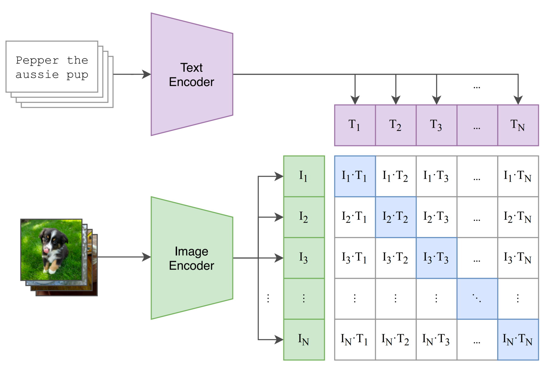
For a batch of \(N\) aligned pairs \((x_n,y_n)\), define similarities: \[ s_{ij}=\frac{f_I(x_i)^\top f_T(y_j)}{\tau} \]

Symmetric contrastive objective: \[ \mathcal{L}_{\text{img}}=-\frac{1}{N}\sum_{i=1}^N \log \frac{e^{s_{ii}}}{\sum_j e^{s_{ij}}}, \quad \mathcal{L}_{\text{text}}=-\frac{1}{N}\sum_{i=1}^N \log \frac{e^{s_{ii}}}{\sum_j e^{s_{ji}}} \] \[ \mathcal{L}_{\text{CLIP}}=\frac{1}{2}\left(\mathcal{L}_{\text{img}}+\mathcal{L}_{\text{text}}\right) \]

Why it mattered:

Uses natural language descriptions instead of only class labels.
Scales to web-scale image-text data.
Enables strong zero-shot transfer.

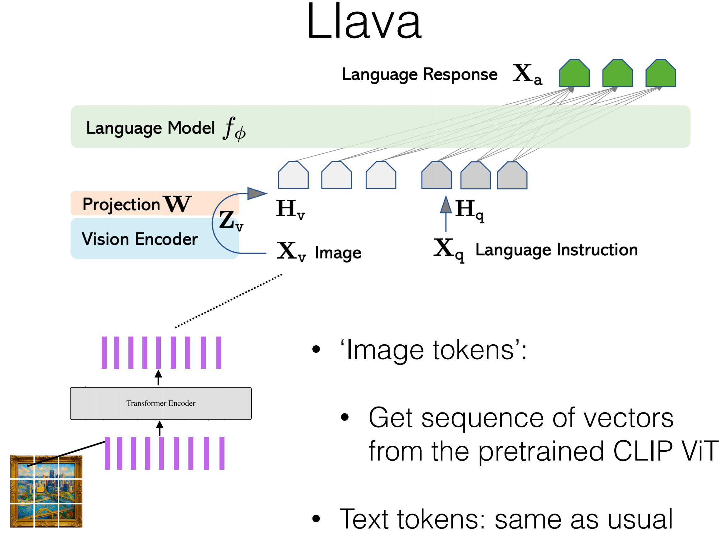
LLaVA-style Combination with a Language Model

General pipeline from lecture:

Preprocess image (patching/cropping).
Encode image with a vision encoder (often CLIP ViT).
Linearly project vision features to LM embedding dimension.
Concatenate visual tokens with text tokens.
Train/fine-tune on image-text instruction data.
For image positions, skip token-level LM loss.

A simple form: \[ h_v=\text{Proj}(f_I(x_{\text{image}})), \quad p_\theta(y_t\mid y_{<t},x_{\text{text}},h_v) \]

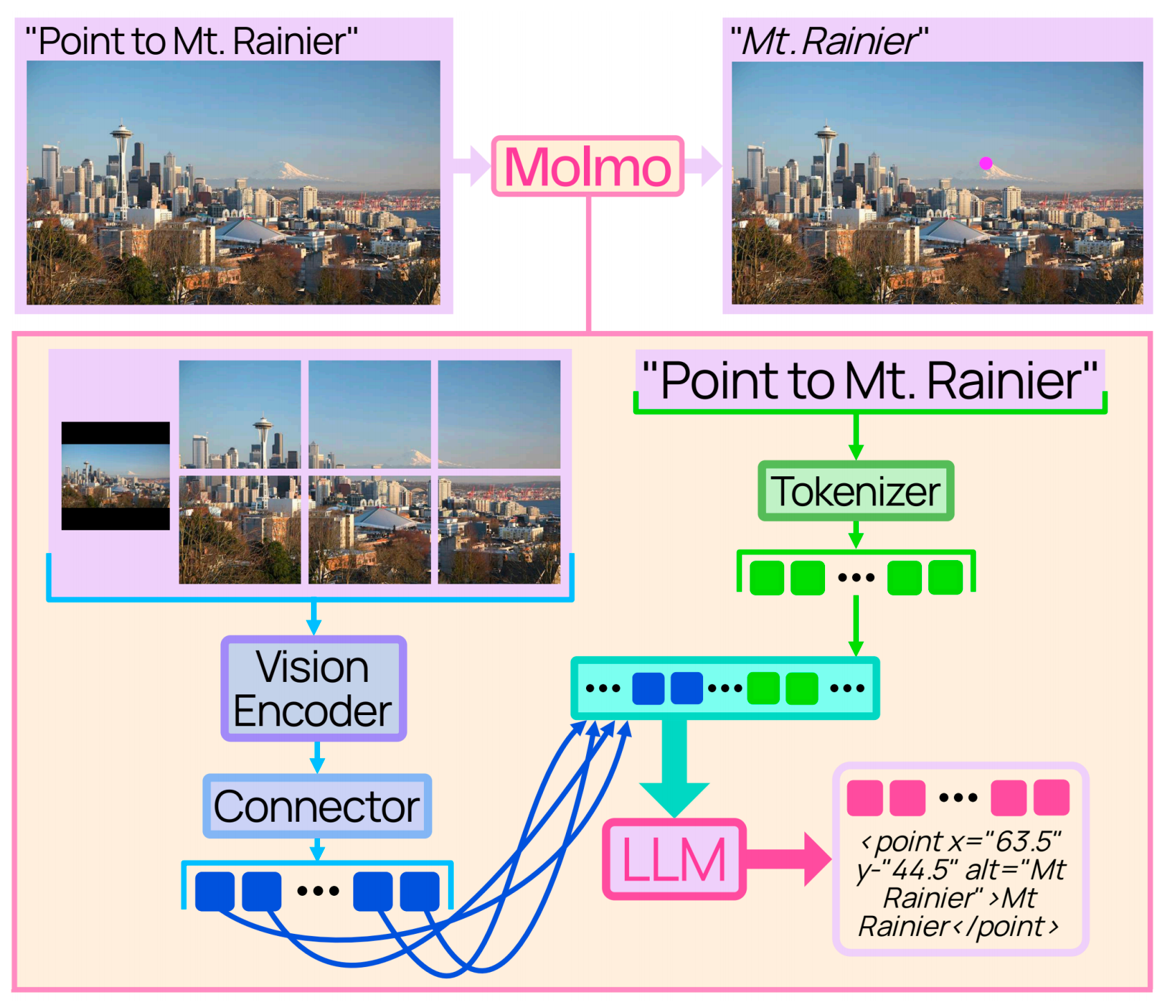
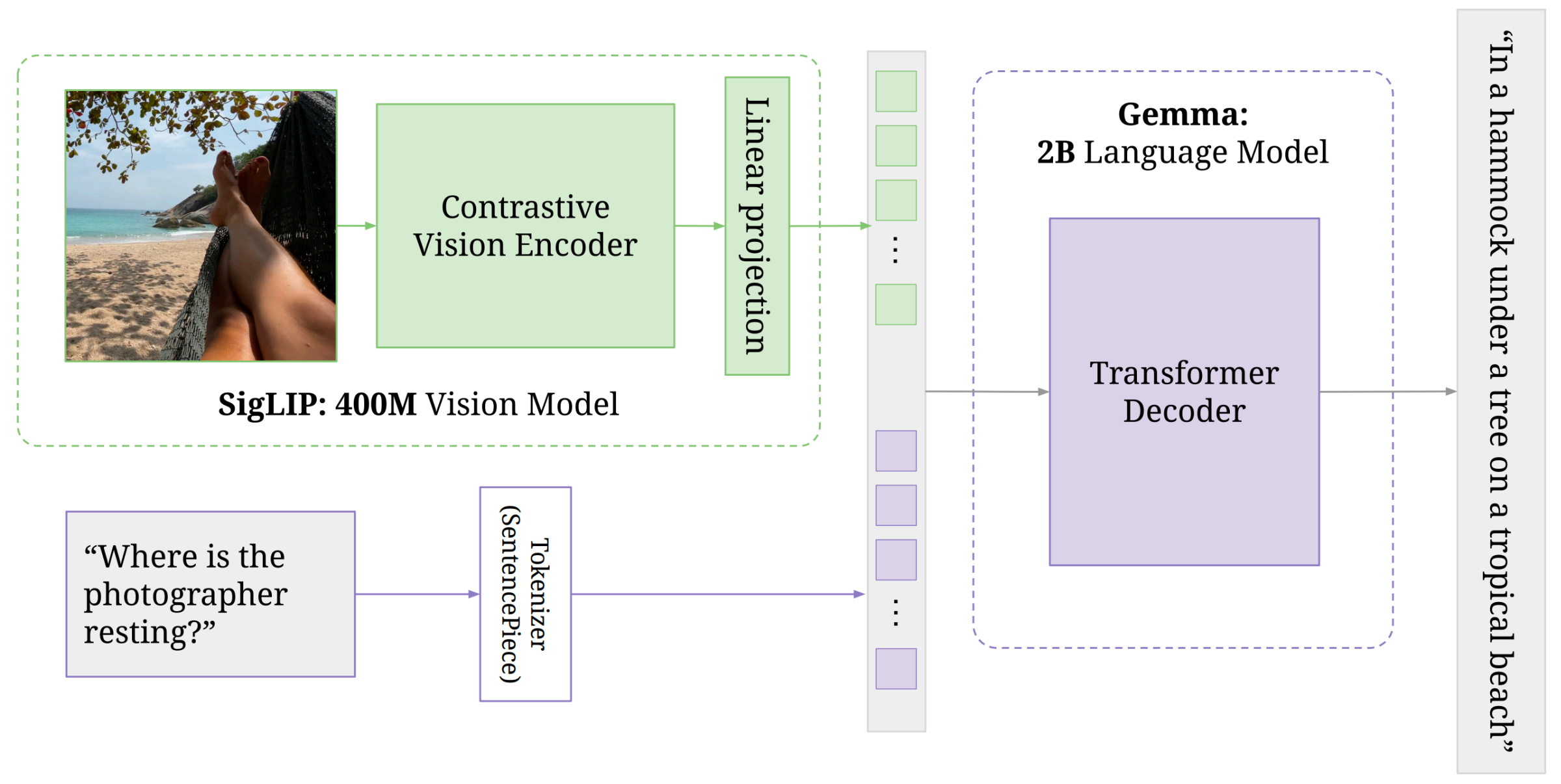
Case Notes Mentioned in Lecture

Molmo (AI2): CLIP ViT-L/14 (336px), then pooling/projection before feeding LM; uses full image + crops.

PaliGemma (Google): lecture highlighted that jointly updating vision encoder + LM can outperform freezing one side.

Lec11 Takeaways

ViT gives a clean tokenization interface for images.
CLIP gives strong, scalable image representations through contrastive learning.
Multimodal assistants are mostly about interface design between vision tokens and LM tokens.

Lec12 Multimodal Modeling II (Generating Images)

Generative Paradigms

Lecture compared four families:

Autoregressive (AR): model \(p(x_t\mid x_{<t})\).
VAE: encode to latent \(z\), decode back.
GAN: generator vs discriminator game.
Diffusion: denoise from noise to data.

Attempt 1: Pixel-level Autoregression

Flatten image into a long sequence of pixel values: \[ x_{\text{img}} \rightarrow (x_1,\dots,x_T),\quad x_t\in\{0,\dots,255\} \] \[ \mathcal{L}_{\text{MLE}}=-\sum_{t=1}^{T}\log p_\theta(x_t\mid x_{<t}) \]

Examples discussed: PixelRNN, Image Transformer, iGPT.

Main bottlenecks:

Sequence length explodes (e.g., \(1024\times1024\times3\approx 3\)M tokens).
Pixel tokens are low-level; learning semantics is data-hungry.

Attempt 2: Learn Discrete Image Tokens

Core idea: learn an image tokenizer/de-tokenizer so the LM models a shorter, semantic token sequence.

VAE Refresher

Standard objective: \[ \mathcal{L}_{\text{VAE}}(x)= -\mathbb{E}_{q_{\theta_{\text{enc}}}(z\mid x)}[\log p_{\theta_{\text{dec}}}(x\mid z)] +D_{\text{KL}}\!\left(q_{\theta_{\text{enc}}}(z\mid x)\|p(z)\right) \]

Equivalent view via ELBO: \[ \log p(x)\ge \mathbb{E}_{q(z\mid x)}[\log p(x\mid z)] -D_{\text{KL}}(q(z\mid x)\|p(z)) \]

VQ-VAE: Continuous to Discrete

Encoder gives continuous latent: \[ z_e(x)\in\mathbb{R}^{d} \]

Quantize by nearest codebook entry: \[ k^*=\arg\min_j\|z_e(x)-e_j\|_2,\quad z_q(x)=e_{k^*} \]

Train with reconstruction + codebook + commitment terms: \[ \mathcal{L}= -\log p(x\mid z_q(x)) +\|\text{sg}[z_e(x)]-e\|_2^2 +\beta\|z_e(x)-\text{sg}[e]\|_2^2 \]

Then model discrete image tokens autoregressively.

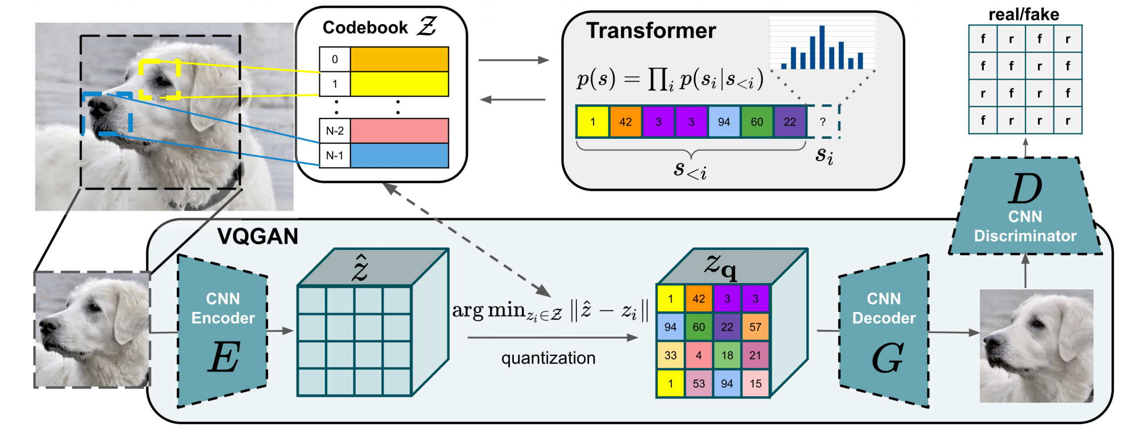
VQ-GAN

VQ-GAN improves VQ-VAE by adding adversarial/perceptual signals in tokenizer training, then training an AR Transformer on resulting token sequences.

Practical gain from lecture:

Sequence becomes much shorter (example: \(32\times32=1024\) tokens) than raw pixels.
Better tradeoff between generation quality and AR modeling feasibility.

Unifying Text and Image Tokens

After tokenizer training:

Add image tokens to LM vocabulary.
Train/fine-tune on mixed text+image token streams.
Decode image tokens back to pixels using de-tokenizer.

Examples discussed: DALL-E (2021), Chameleon (Meta, 2024).

Lec12 Takeaways

Pure pixel AR is conceptually simple but hard to scale.
Discrete tokenizers (VQ-VAE/VQ-GAN) are the key bridge for AR multimodal models.
Tradeoff: unified token modeling vs information loss from tokenization.

Lec15 Multimodal Modeling III (Diffusion and Flows)

Where This Fits

The first two multimodal lectures covered:

multi-to-text: encode images into token-like representations for an LM
token-based multi-to-image: generate images through discrete visual tokens

This lecture moves to the dominant modern paradigm for text-to-image systems:

start from noise
iteratively denoise toward an image
condition the process on text (and potentially other modalities)

Stable Diffusion 3 is a canonical example of this style.

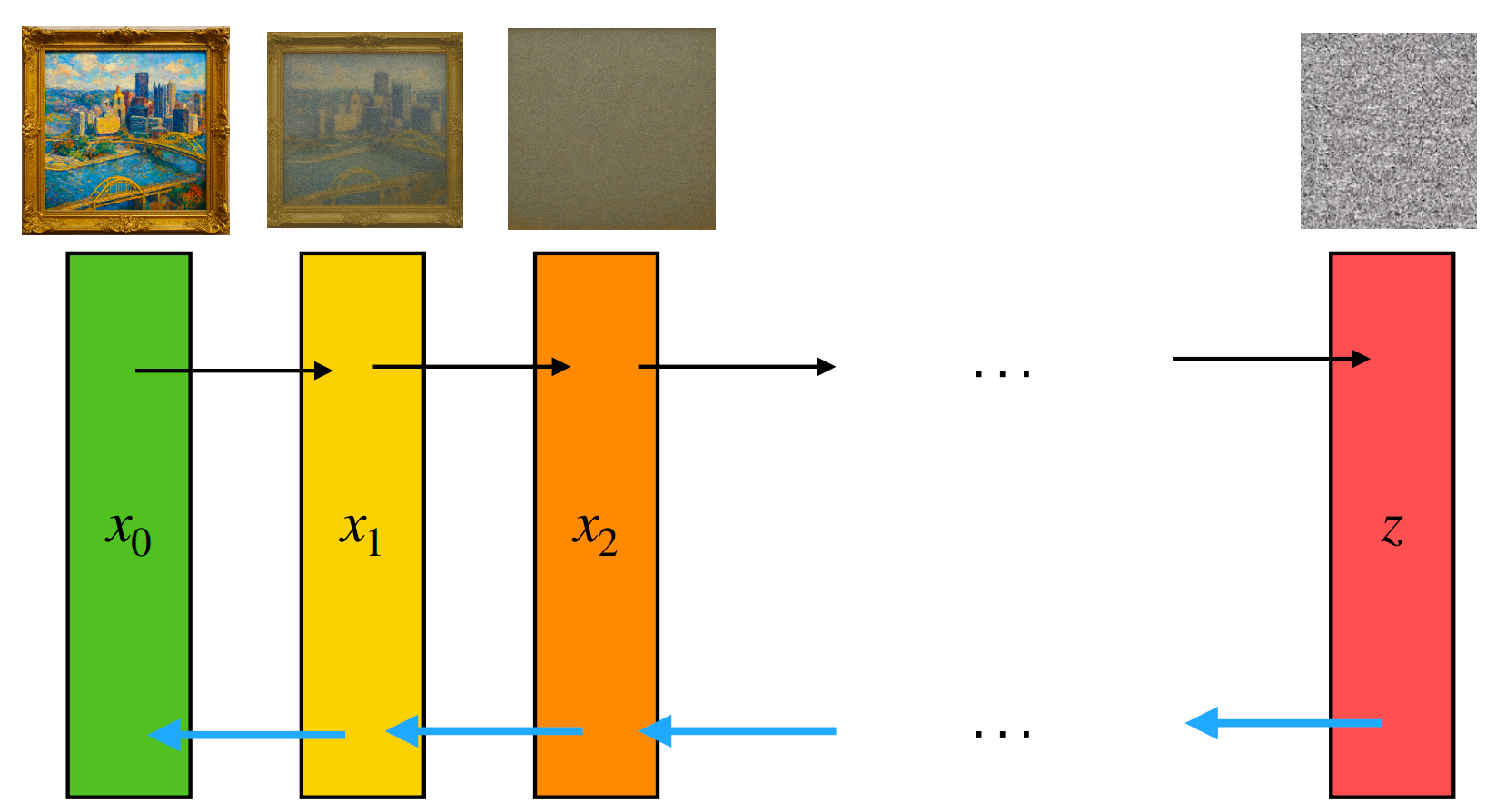
Diffusion: Core Idea

Diffusion models define a fixed forward noising process and a learned reverse denoising process.

Forward process: \[ q(x_t \mid x_{t-1}) = \mathcal{N}\!\left(x_t;\sqrt{\alpha_t}\,x_{t-1}, (1-\alpha_t)I\right) \]

Let \(\beta_t = 1-\alpha_t\) and \(\bar{\alpha}_t=\prod_{i=1}^t \alpha_i\). Then we can sample directly from \(x_0\): \[ q(x_t \mid x_0) = \mathcal{N}\!\left(x_t;\sqrt{\bar{\alpha}_t}\,x_0,(1-\bar{\alpha}_t)I\right) \] \[ x_t=\sqrt{\bar{\alpha}_t}\,x_0+\sqrt{1-\bar{\alpha}_t}\,\epsilon, \quad \epsilon \sim \mathcal{N}(0,I) \]

Noise schedule requirements from lecture:

\(\bar{\alpha}_0 = 1\) so we start with data
\(\bar{\alpha}_T \approx 0\) so we end close to pure noise
the schedule should decrease monotonically

A common choice is a linear schedule for \(\beta_t\).

Training DDPM

In principle, the model maximizes \(\log p_\theta(x_0)\) through an ELBO over latent variables \(x_{1:T}\).
The ELBO decomposes into:

prior matching at the final noisy step
denoising terms that match each reverse transition
a reconstruction term near \(x_0\)

The practical training objective from the lecture is the simplified noise-prediction loss: \[ \mathcal{L}_{\text{simple}}(\theta)= \mathbb{E}_{x_0,\epsilon,t} \left[\left\|\epsilon-\epsilon_\theta(x_t,t)\right\|_2^2\right], \quad t \sim \text{Uniform}\{1,\dots,T\} \]

Training loop:

sample a real image \(x_0\)
sample timestep \(t\)
sample Gaussian noise \(\epsilon\)
construct \(x_t\)
train the network to recover the injected noise

Sampling

The learned reverse process starts from noise: \[ x_T \sim \mathcal{N}(0,I) \]

Then for \(t=T,\dots,1\), use \(\epsilon_\theta(x_t,t)\) to parameterize \[ p_\theta(x_{t-1}\mid x_t) \] and sample the next less-noisy state. Repeating this process gradually converts noise into an image.

DDPM as Score Learning

Lecture made an important connection between noise prediction and score estimation.

Write the noisy variable as: \[ z_t = a_t x_0 + \sigma_t \epsilon \]

The score of the marginal distribution is: \[ \nabla_{z_t} \log p(z_t) \]

For this Gaussian corruption process, the expected noise satisfies: \[ \bar{\epsilon} = -\sigma_t \nabla_{z_t}\log p(z_t) \]

Since DDPM trains \(\epsilon_\theta(z_t,t)\) to approximate the true injected noise, the optimal predictor satisfies: \[ \epsilon_\theta(z_t,t)\approx -\sigma_t \nabla_{z_t}\log p(z_t) \]

So DDPM implicitly learns the score function. Intuitively:

predicting the noise tells the model how to remove corruption
removing corruption moves samples toward higher-probability regions

Conditional Generation and Guidance

To generate from a prompt or label \(c\), we need a conditional model.

Classifier Guidance

If we have an auxiliary classifier \(p_\phi(c \mid z_t)\), then we can modify the denoising prediction with the classifier gradient: \[ \tilde{\epsilon}_{\theta,\phi}(z_t,c) = \epsilon_\theta(z_t,c)-w\sigma_t \nabla_{z_t}\log p_\phi(c\mid z_t) \]

The extra term pushes sampling toward images more compatible with condition \(c\).

Classifier-Free Guidance

Instead of training a separate classifier, train one model both with and without conditioning, then combine the two predictions at sampling time: \[ \tilde{\epsilon}_\theta(z_t,c) = (1+w)\epsilon_\theta(z_t,c)-w\epsilon_\theta(z_t) \]

This is the standard practical recipe in modern diffusion systems.
Larger guidance weight \(w\) usually improves prompt alignment, but often reduces diversity.

Important Extensions

The lecture highlighted several common extensions:

Problem	Solution	Main idea
Pixel-space diffusion is expensive	Latent diffusion	Run diffusion in an autoencoder latent space
U-Net inductive bias may be limiting	Diffusion Transformer (DiT)	Replace convolution-heavy backbone with a Transformer
Reverse process can be stochastic and slow	Continuous-time / ODE views	Use deterministic paths and better solvers
Sampling still takes many steps	Distillation	Train a student sampler with fewer steps

These are the main reasons modern systems are much more practical than the original pixel-space DDPM setup.

Continuous-Time View

As the number of steps goes to infinity, diffusion can be described as a stochastic differential equation (SDE): \[ dz = f(t)z\,dt + g(t)\,dw \]

The reverse-time SDE becomes: \[ dz= \left[f(t)z-g(t)^2 \nabla_z \log p_t(z)\right]dt + g(t)\,d\bar{w} \]

Because DDPM estimates the score, we can plug in: \[ \nabla_z \log p_t(z)\approx -\frac{\epsilon_\theta(z,t)}{\sigma_t} \]

There is also a deterministic probability-flow ODE with the same marginals: \[ dz= \left[f(t)z-\frac{1}{2}g(t)^2 \nabla_z \log p_t(z)\right]dt \]

This viewpoint matters because it connects diffusion to numerical ODE solvers and motivates alternative generation methods.

Flow Matching

Flow matching keeps the idea of transporting one distribution into another, but formulates the problem more directly as learning a velocity field.

Let:

\(p_0\) be a simple source distribution such as Gaussian noise
\(p_1\) be the target data distribution
\(v_t(\cdot)\) be a time-dependent velocity field

The flow \(\phi_t\) is defined by the ODE: \[ \frac{d}{dt}\phi_t(x)=v_t(\phi_t(x)), \quad \phi_0(x)=x \]

If \(v_t\) is correct, pushing \(X_0 \sim p_0\) through this ODE gives \(X_1 \sim p_1\).

Conditional Flow Matching

For a single data point \(x_1\), lecture used the straight-line path: \[ X_t = (1-t)X_0 + t x_1 \]

Its velocity is known exactly: \[ \frac{d}{dt}X_t = x_1 - X_0 \]

So training becomes: \[ \mathcal{L}_{\text{CFM}} = \mathbb{E}_{x_1,X_0,t} \left[\left\|v_\theta(X_t,t)-(x_1-X_0)\right\|_2^2\right] \]

Key intuition:

diffusion learns how to denoise a corrupted point
flow matching learns how to move along a transport path

Compared with DDPM, flow matching often gives straighter trajectories and can be integrated in fewer steps.

Case Study: Stable Diffusion 3

Lecture used Stable Diffusion 3 as a modern example:

Flow matching: replaces the classic DDPM-style training target
Latent space: operates on the latent space of a pretrained autoencoder
Text conditioning: combines CLIP text features with T5 features

The broader lesson is that state-of-the-art text-to-image systems are now hybrids:

latent-space modeling for efficiency
strong text encoders for conditioning
Transformer-style backbones and ODE/flow-inspired training for better generation quality

Lec15 Takeaways

DDPM trains a model to reverse a fixed noising process.
Noise prediction is closely tied to score estimation.
Guidance makes diffusion usable for conditional generation.
Continuous-time views connect diffusion to ODE solvers.
Flow matching is a cleaner transport-based alternative that now powers systems like Stable Diffusion 3.

Final Summary

Lec11: how to encode images for text generation (ViT + CLIP + LM integration).
Lec12: how to generate images with token-based generative modeling.
Lec15: how modern text-to-image systems generate images by denoising or transporting noise into data.
Together they frame multimodal systems as: representation (encode) + alignment (shared space) + generation (discrete or continuous).

This post is based on CMU 11-711 Advanced NLP lecture materials (Multimodal Modeling I, II, and III, Sean Welleck).