Lec10 Retrieval and RAG

Why Retrieval?

Large language models are powerful, but they still suffer from:

Hallucination: generating fluent but unsupported claims.
Stale knowledge: model parameters cannot instantly reflect new facts.
Monolithic memory bottleneck: all knowledge is compressed into fixed parameters.

Retrieval-augmented systems treat external documents as a non-parametric memory and fetch evidence at inference time.

Retrieval-Augmented LM: Core Intuition

Given a query $x$:

Retrieve top-$k$ relevant passages from a datastore.
Feed retrieved passages + query to the generator.
Generate an answer grounded in retrieved evidence.

Key components:

Datastore: the corpus and index.
Retriever: maps query/document to similarity scores.
Generator (LM): produces final response.

Part 1: Datastore

What to Store?

Typical options include:

Web pages, papers, wiki pages, domain documents.
Passage-level chunks instead of full documents.
Metadata (source, timestamp, URL, section title) for attribution and filtering.

Processing Pipeline

A practical pipeline:

Curation: pick sources relevant to target tasks.
Preprocessing: HTML/PDF to clean text, normalize, deduplicate.
Chunking: split long docs into passages.
Indexing: build sparse or dense retrieval index.

Chunking trade-off:

Too short: lacks context.
Too long: introduces noise and hurts retrieval precision.

Scaling Considerations

Corpus size can reach billions of tokens or more.
Use ANN index and sharding for low-latency serving.
Keep document freshness via periodic re-indexing.

Part 2: Retriever

Sparse Retriever (TF-IDF / BM25)

Classic lexical matching uses bag-of-words style vectors.

TF-IDF basics: \[ \text{TF}(t, d)=\frac{\text{freq}(t,d)}{\sum_{t'} \text{freq}(t',d)}, \quad \text{IDF}(t)=\log\frac{N}{\text{df}(t)} \]

TF(t, d) measures how frequently term $t $ appears in document $d $, normalized by document length.
IDF(t) measures how rare a term is across the entire corpus. Common words like “the” appear in nearly every document, so $(t) N $ and IDF → 0.
The final TF-IDF score is simply $(t,d) (t) $: a term matters most when it’s frequent in this document but rare globally.

BM25 score: \[ \text{BM25}(q,d)=\sum_{t \in q} \text{IDF}(t)\cdot \frac{\text{TF}(t,d)(k_1+1)} {\text{TF}(t,d)+k_1\left(1-b+b\frac{|d|}{\text{avgdl}}\right)} \]

BM25 (Best Matching 25) is a probabilistic refinement of TF-IDF, and is the default ranking function in search engines like Elasticsearch and Lucene. Two key improvements:

TF saturation (controlled by $k_1 $, typically 1.2): As $(t,d) $ grows, the score approaches an asymptotic limit of $(k_1 + 1) $. This prevents a document from dominating just because it repeats a keyword excessively. In contrast, raw TF-IDF grows linearly without bound.
Document length normalization (controlled by $b $, typically 0.75): The term $b $ penalizes longer documents, since they naturally have higher term frequencies. When $b = 0 $, no length normalization is applied; when $b = 1 $, full normalization relative to the average document length (avgdl).

Pros:

Fast and strong lexical precision.
No neural training needed.

Cons:

Weak semantic matching for paraphrases.

Dense Retriever (Bi-Encoder)

Encode query and documents into dense vectors: \[ s(q,d)=\langle E_q(q), E_d(d) \rangle \]

Common training uses contrastive learning: \[ \mathcal{L}= -\log \frac{\exp(s(q,d^+)/\tau)} {\exp(s(q,d^+)/\tau)+\sum_{d^-}\exp(s(q,d^-)/\tau)} \]

Pros:

Better semantic retrieval.
Works for paraphrases and lexical mismatch.

Cons:

Requires training data and ANN infrastructure.

Fast Nearest Neighbor Search

Dense retrieval at scale relies on approximate nearest neighbor (ANN) methods (e.g., FAISS) to trade tiny recall loss for large latency gains.

Re-ranking with Cross-Encoder

Two-stage retrieval is common:

Bi-encoder retrieves top-$k$ candidates quickly.
Cross-encoder re-ranks the shortlist with higher accuracy.

Evaluation Metrics and Benchmarks

Frequent metrics:

Recall@k: whether relevant docs are found in top-$k$.
MRR: reciprocal rank quality for first relevant hit.
nDCG@k: graded ranking quality.
Precision@k: fraction of top-$k$ hits that are relevant.

Benchmarks highlighted in lecture:

BEIR (zero-shot IR across heterogeneous tasks).
MTEB (massive embedding benchmark).

Part 3: How to Use Retrieval

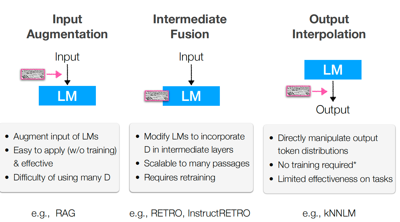
In-contet RAG (Input Augmentation)

Retrieve evidence and append it to prompt context.

Sequence-level RAG form: \[ p(y \mid x) \approx \sum_{z \in \text{top-}k} p_\eta(z \mid x)\,p_\theta(y \mid x, z) \]

Token-level marginalization form: \[ p(y \mid x) \approx \prod_i \sum_{z \in \text{top-}k} p_\eta(z \mid x)\,p_\theta(y_i \mid x, z, y_{<i}) \]

Training Strategies for RAG

Independent training: train retriever and generator separately.
Sequential training: train retriever first, then adapt generator.
End-to-end training: optimize retrieval and generation jointly.

Limitations of In-context RAG

Retrieval can return irrelevant passages (error propagation).
Long contexts increase cost and may dilute useful evidence.
Generator may still ignore retrieved evidence if prompts are weak.

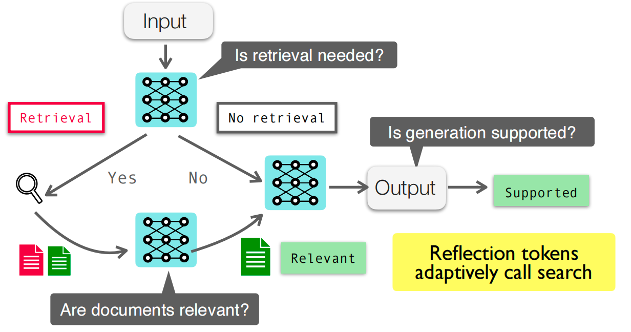
Self-RAG and Adaptive Retrieval

Self-RAG style systems learn to:

Decide whether retrieval is needed.
Decide when to retrieve again during generation.
Critique or verify generation quality with evidence.

This makes retrieval usage conditional rather than always-on.

Beyond In-context RAG

Tool-augmented LMs: invoke tools/search APIs iteratively.
Deep Research Agents: multi-step retrieval + synthesis workflows.
Intermediate augmentation: RETRO / kNN-LM retrieve at hidden-state or token level, not only prompt level.

Practical Checklist

Define target domain and freshness requirement.
Build clean, well-chunked datastore with metadata.
Choose sparse/dense/hybrid retrieval based on latency-quality budget.
Add reranker if top-$k$ quality is bottleneck.
Track retrieval metrics and end-task accuracy jointly.
Add citation and evidence checks to reduce hallucination risk.

Key Takeaways

RAG adds an external, updatable memory to LMs.
Quality depends on three coupled parts: datastore, retriever, generator.
Dense retrieval + reranking is often the practical high-performance path.
Adaptive retrieval (Self-RAG, tool use) addresses limits of static in-context RAG.