15642 Machine Learning Systems: Distributed Training and Parallelization
Data Parallelism and Zero Redundancy
Course: 15-442/15-642 Machine Learning Systems Instructors: Tianqi Chen and Zhihao Jia Carnegie Mellon University
DNN Training Overview
DNN training iterates three phases: forward propagation computes layer outputs \(h^{(l+1)} = f^{(l)}(W^{(l)} h^{(l)} + b^{(l)})\), backward propagation computes gradients via chain rule \(\frac{\partial L}{\partial W^{(l)}}\), and weight update applies \(W^{(l)} \leftarrow W^{(l)} - \eta \frac{\partial L}{\partial W^{(l)}}\).
Each GPU must store parameters, activations (saved for backward), gradients, and optimizer states (e.g., momentum and variance for Adam). For large models, this memory footprint becomes the primary bottleneck.
Data Parallelism Basics
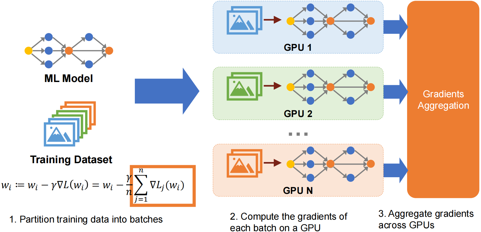
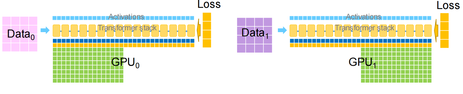
Data parallelism splits training data across multiple workers (GPUs), each holding a full copy of the model. The training loop per iteration:
- Scatter data: Distribute different mini-batches to each worker
- Forward & Backward: Each worker independently computes gradients on its local data
- Synchronize gradients: Aggregate gradients across all workers (AllReduce)
- Update parameters: Each worker applies the optimizer step with aggregated gradients
All workers maintain identical parameters through synchronized gradient updates. With 4 workers and batch size 32, each processes 8 samples — ideally 4x speedup.
Gradient Aggregation Strategies
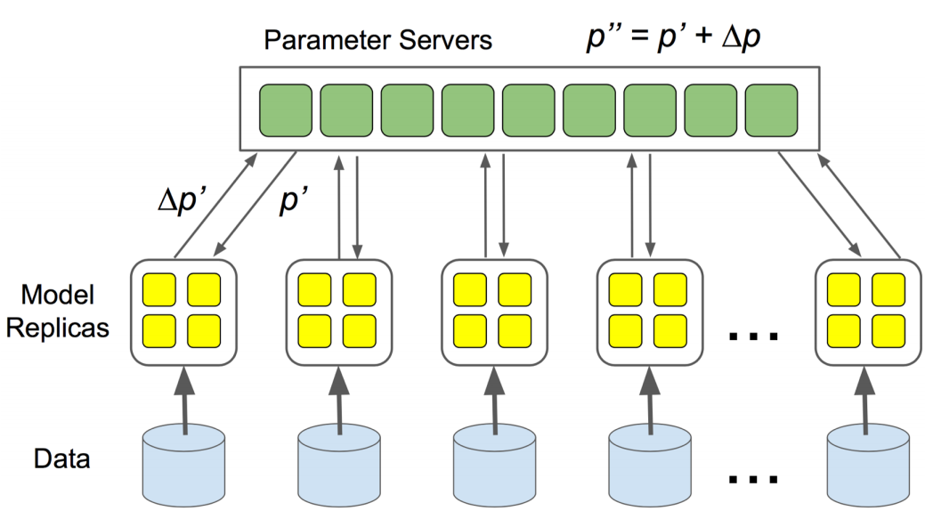
Parameter Server Architecture
The Parameter Server is a centralized approach: workers push gradients to a central server (\(N \times M\) communication), the server aggregates and updates parameters, then workers pull the updated weights (\(N \times M\) communication). Total communication: \(2NM\) per iteration.
Limitations: All traffic funnels through the server, creating a bandwidth bottleneck that worsens with more workers. It is also a single point of failure with uneven load distribution. This architecture does not scale well.
AllReduce Communication Patterns
AllReduce is a decentralized collective operation: all workers contribute local gradients and receive the aggregated result. No single bottleneck node.
Naive AllReduce
Every worker broadcasts its \(M\) parameters to all \((N-1)\) others. Total communication: \(N(N-1)M = O(N^2 M)\) — quadratic scaling, not efficient.
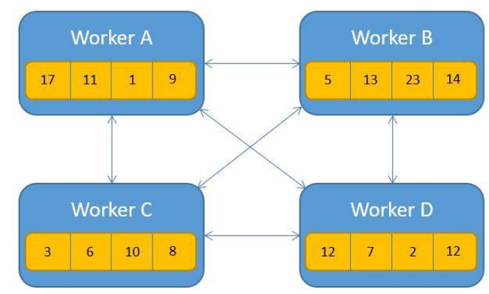
Ring AllReduce
Ring AllReduce achieves optimal communication complexity by organizing workers in a logical ring.
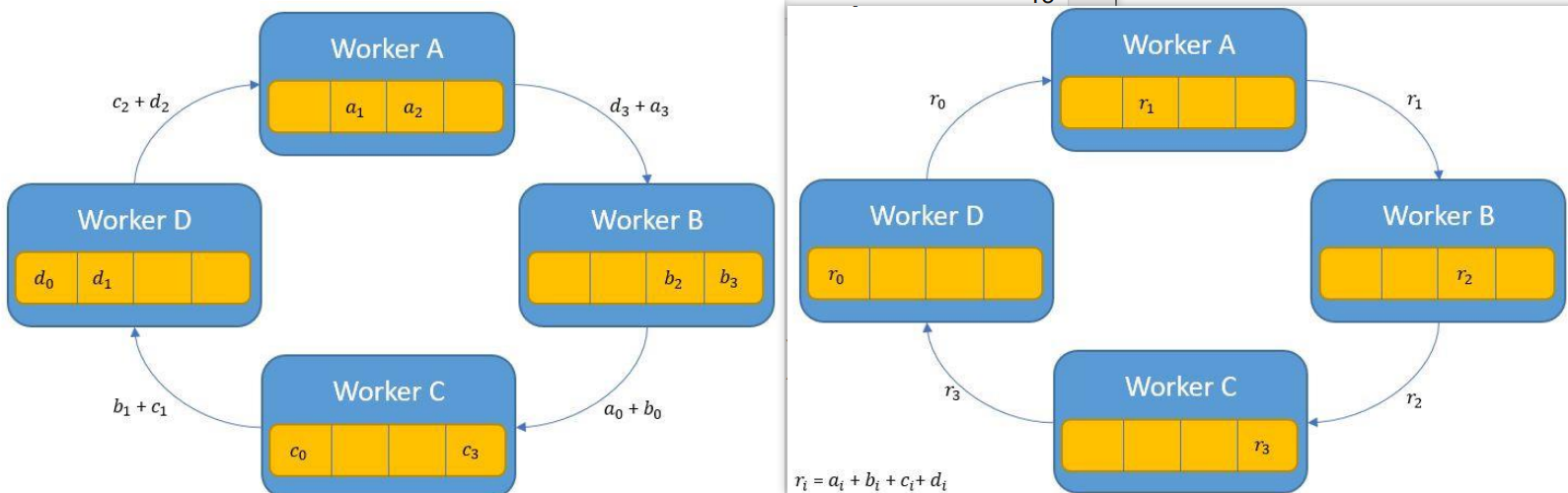
Aggregation Phase
Setup: Arrange N workers in a ring: \(W_0 \leftrightarrow W_1 \leftrightarrow \cdots \leftrightarrow W_{N-1} \leftrightarrow W_0\)
Strategy: Partition parameters into N chunks, process one chunk per step.
Process (N-1 steps):
- Each worker starts with one chunk as “responsible chunk”
- Step k \((k = 0, 1,
\ldots, N-2)\):
- Worker \(i\) sends chunk \(j\) to worker \((i+1) \mod N\)
- Worker \(i\) receives chunk \(j'\) from worker \((i-1) \mod N\)
- Worker \(i\) accumulates received chunk: \(\text{chunk}_{j'} \leftarrow \text{chunk}_{j'} + \text{received}\)
Result: After N-1 steps, each worker has the fully aggregated result for one chunk.
Broadcast Phase
Goal: Distribute the aggregated chunks so every worker has all chunks.
Process (N-1 steps):
- Step k \((k = 0, 1,
\ldots, N-2)\):
- Worker \(i\) sends its completed chunk to worker \((i+1) \mod N\)
- Worker \(i\) receives a completed chunk from worker \((i-1) \mod N\)
Result: After N-1 steps, all workers have all aggregated chunks.
Communication Cost Analysis
Each step transfers \(M/N\) per worker. Total steps: \(2(N-1)\) (N-1 aggregation + N-1 broadcast).
Total per worker: \(2(N-1) \times \frac{M}{N} \approx 2M\) — independent of N, optimal scaling.
Total network communication: \(2(N-1)M \approx 2NM\).
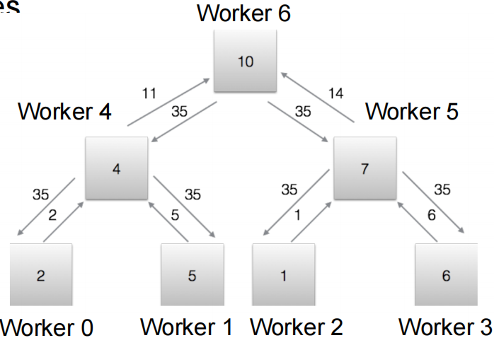
Tree AllReduce
Workers form a binary tree with depth \(\log_2 N\). The Reduce phase (bottom-up) aggregates gradients from leaves to root; the Broadcast phase (top-down) distributes the result back.
Communication: Reduce phase \(\sum_{i=1}^{\log_2 N} \frac{N}{2^i} \times M = (N-1)M\), broadcast phase \((N-1)M\). Total: \(2(N-1)M \approx 2NM\) in only \(2\log_2 N\) iterations (fewer than ring’s \(2(N-1)\)). Trade-off: potential bandwidth bottleneck at the root.
Butterfly AllReduce
Uses a hypercube-based pattern: in iteration \(k\), worker \(i\) communicates with worker \(i \oplus 2^k\) (XOR). For 8 workers: iteration 0 pairs 0↔︎1, 2↔︎3, 4↔︎5, 6↔︎7; iteration 1 pairs 0↔︎2, 1↔︎3, 4↔︎6, 5↔︎7; iteration 2 pairs 0↔︎4, 1↔︎5, 2↔︎6, 3↔︎7.
Each iteration, workers exchange \(M/2\) parameters with their partner and aggregate locally. All workers operate in parallel with balanced load.
Communication: \(M\) per worker per iteration × \(\log_2 N\) iterations = \(NM\log_2 N\) total. Slightly more than Ring/Tree (\(2NM\)), but only \(\log_2 N\) iterations — best when latency matters more than total bandwidth. Requires power-of-2 worker count.

Performance Comparison
| Algorithm | Total Communication | Iterations | Bandwidth Bottleneck |
|---|---|---|---|
| Parameter Server | \(2NM\) | 2 | Server bottleneck |
| Naive AllReduce | \(N(N-1)M\) | 1 | Quadratic scaling |
| Ring AllReduce | \(2NM\) | \(2(N-1)\) | Balanced |
| Tree AllReduce | \(2NM\) | \(2\log_2 N\) | Root bottleneck |
| Butterfly AllReduce | \(NM\log_2 N\) | \(\log_2 N\) | Balanced |
Ring AllReduce is the most commonly used in practice (PyTorch DDP, Horovod) — optimal \(2NM\) communication with balanced bandwidth. Tree AllReduce trades root bottleneck risk for fewer iterations (\(2\log_2 N\)). Butterfly minimizes iterations (\(\log_2 N\)) at the cost of slightly higher total communication.

Large Model Training Challenges
As models scale to billions of parameters, memory becomes the critical bottleneck.
Memory Breakdown
For a model with M parameters using mixed-precision training with Adam:
| Component | Precision | Memory |
|---|---|---|
| Parameters | FP16 | \(2M\) bytes |
| Gradients | FP16 | \(2M\) bytes |
| Optimizer: FP32 master copy | FP32 | \(4M\) bytes |
| Optimizer: Momentum (1st moment) | FP32 | \(4M\) bytes |
| Optimizer: Variance (2nd moment) | FP32 | \(4M\) bytes |
| Total | \(16M\) bytes |
FP16 is used for forward/backward computation (faster, less memory). FP32 is required for optimizer updates to prevent numerical errors during accumulation.

Scaling Examples
| Model | Parameters | Training Memory | Hardware |
|---|---|---|---|
| BERT-Large (2018) | 340M | 5.4 GB | Fits on single V100 (16GB) |
| GPT-2 (2019) | 1.5B | 24 GB | Requires multi-GPU |
| GPT-3 (2020) | 175B | 2.8 TB | 35+ A100-80GB GPUs |
Standard data parallelism replicates the full model on each GPU — massive memory redundancy.
ZeRO: Zero Redundancy Optimizer
Overview
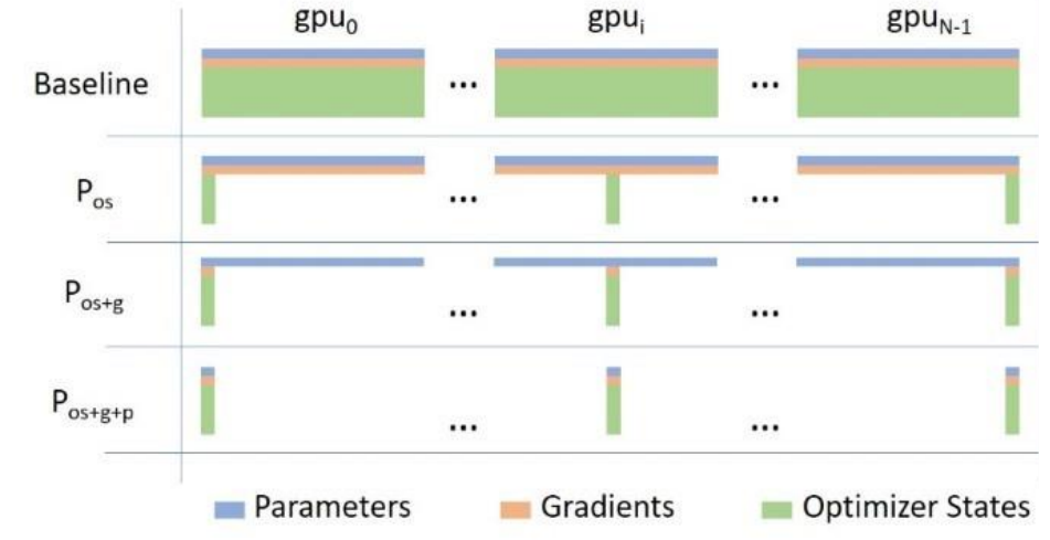
ZeRO (Zero Redundancy Optimizer) eliminates memory redundancy in data-parallel training. Standard DP replicates parameters, gradients, and optimizer states on every GPU — for N GPUs, that is N copies of everything, wasting \((N-1) \times 16M\) bytes.
ZeRO’s idea: partition these components across GPUs instead of replicating them, reducing per-GPU memory from \(16M\) to \(\frac{16M}{N}\) at the cost of additional communication.
ZeRO Stage 1: Partitioning Optimizer States
ZeRO-1 partitions only the optimizer states across GPUs. Parameters and gradients remain fully replicated. Each GPU is responsible for updating only its assigned \(\frac{1}{N}\) partition.
Training iteration: 1. Forward: Normal computation using full local parameters (no communication) 2. Backward: Compute full gradients → AllReduce to synchronize (\(2M\) communication) 3. Weight Update: Each GPU updates only its partition using local optimizer states 4. Parameter Sync: AllGather to reconstruct full parameters on every GPU (\(2M\) communication)
Memory per GPU: \(4M + \frac{12M}{N}\) (parameters \(2M\) + gradients \(2M\) + partitioned optimizer \(\frac{12M}{N}\))
Communication: \(4M\) per iteration. For N=4: memory = \(7M\) vs baseline \(16M\) — 2.3x reduction.
ZeRO Stage 2: Partitioning Gradients
ZeRO-2 additionally partitions gradients — since each GPU only needs gradients for the parameters it updates, there is no need for a full gradient buffer.
The key change: replace AllReduce with Reduce-Scatter during backward. Reduce-Scatter aggregates gradients but only delivers each GPU the partition it owns (no broadcast phase needed). This can happen layer-by-layer during backpropagation, overlapping communication with computation.
Training iteration: 1. Forward: Normal computation (no communication) 2. Backward: Compute gradients → Reduce-Scatter per layer, each GPU keeps only its partition 3. Weight Update: Each GPU updates its partition 4. Parameter Sync: AllGather to reconstruct full parameters (\(2M\))
Memory per GPU: \(2M + \frac{14M}{N}\) (parameters \(2M\) + partitioned gradients \(\frac{2M}{N}\) + partitioned optimizer \(\frac{12M}{N}\))
Communication: \(4M\) per iteration (same as ZeRO-1). For N=4: memory = \(5.5M\) — 2.9x reduction.

ZeRO Stage 3: Partitioning Parameters
ZeRO-3 partitions everything — no component is replicated. Each GPU stores only \(\frac{1}{N}\) of parameters, gradients, and optimizer states. The challenge: how to compute forward/backward without full parameters? Solution: AllGather parameters on demand, then discard.
Forward (layer-by-layer): AllGather \(W^{(l)}\) → compute layer → discard gathered parameters (keep only own partition and activations).
Backward (layer-by-layer): AllGather \(W^{(l)}\) again → compute gradients → Reduce-Scatter gradients → discard gathered parameters → update own partition immediately.

No separate parameter sync step needed — updated parameters are already correctly partitioned.
Memory per GPU: \(\frac{16M}{N}\) — perfect linear scaling (\(O(M/N)\)).
Communication: \(4M\) per iteration (AllGather in forward \(+\) AllGather in backward \(+\) Reduce-Scatter gradients). This is 2x the baseline, but enables training models that otherwise cannot fit in memory. Use when ZeRO-2 is insufficient.
Performance Analysis
Memory Comparison (M parameters, N GPUs)
| Component | Baseline DP | ZeRO-1 | ZeRO-2 | ZeRO-3 |
|---|---|---|---|---|
| Parameters | \(2M\) | \(2M\) | \(2M\) | \(\frac{2M}{N}\) |
| Gradients | \(2M\) | \(2M\) | \(\frac{2M}{N}\) | \(\frac{2M}{N}\) |
| Optimizer States | \(12M\) | \(\frac{12M}{N}\) | \(\frac{12M}{N}\) | \(\frac{12M}{N}\) |
| Total | \(16M\) | \(4M + \frac{12M}{N}\) | \(2M + \frac{14M}{N}\) | \(\frac{16M}{N}\) |
GPT-3 (175B, 64 GPUs): Baseline = 2.8 TB/GPU (impossible), ZeRO-1 = 750 GB, ZeRO-2 = 481 GB, ZeRO-3 = 44 GB (fits on A100-80GB).
Communication Comparison
| Stage | Forward | Backward | Update | Total |
|---|---|---|---|---|
| Baseline DP | - | \(2M\) (AllReduce) | - | \(2M\) |
| ZeRO-1 | - | \(2M\) (AllReduce) | \(2M\) (AllGather) | \(4M\) |
| ZeRO-2 | - | \(2M\) (Reduce-Scatter) | \(2M\) (AllGather) | \(4M\) |
| ZeRO-3 | \(2M\) (AllGather) | \(2M\) (Reduce-Scatter) | - | \(4M\) |
All ZeRO stages have 2x communication vs baseline. ZeRO-3 has higher latency due to layer-by-layer synchronization but enables the largest models. High-speed interconnects (NVLink, InfiniBand) are essential, and communication can be overlapped with computation to hide latency.
Summary
| Stage | Partitioned | Memory per GPU | Communication |
|---|---|---|---|
| Baseline DP | Nothing | \(16M\) | \(2M\) |
| ZeRO-1 | Optimizer states | \(4M + \frac{12M}{N}\) | \(4M\) |
| ZeRO-2 | Optimizer + Gradients | \(2M + \frac{14M}{N}\) | \(4M\) |
| ZeRO-3 | Everything | \(\frac{16M}{N}\) | \(4M\) |
ZeRO enables linear memory scaling (\(O(M/N)\)) at a modest 2x communication overhead. Used in practice by DeepSpeed and PyTorch FSDP.
Choosing a strategy: Standard DP when the model fits on one GPU; ZeRO-1 when optimizer memory is limiting; ZeRO-2 when gradients also need reduction; ZeRO-3 when even parameters don’t fit.
Note on Memory Model: The notes above use a 16M model (optimizer states = 12M). The Q&A section below uses the 20Ψ model from the ZeRO paper, which explicitly counts the FP32 gradient copy as part of optimizer states (optimizer states = 16Ψ). The 20Ψ model is more precise for mixed-precision training with Adam.
Model Parallelism and Pipeline Parallelism
Model Parallelism Overview
Model parallelism addresses the fundamental limitation of data parallelism: when the model is too large to fit on a single GPU. Instead of replicating the entire model, model parallelism splits the model across multiple devices.
Key idea: Partition the model into multiple subgraphs and assign different subgraphs to different GPUs. Each GPU: - Stores only a portion of the model parameters - Computes forward/backward for its assigned layers - Transfers intermediate activations to the next GPU in the pipeline

This enables training models that exceed single-GPU memory, but introduces new challenges: communication overhead and potential GPU under-utilization.
Tensor Model Parallelism
Tensor model parallelism partitions parameters within a single layer across multiple GPUs. For a matrix multiplication \(y = xW\), we can partition either the output dimension or the input dimension of \(W\).
Partition Output (Column-wise Split)
Split weight matrix \(W\) column-wise: \(W = [W_1, W_2]\)
Each GPU computes a portion of the output independently:
\[ \begin{aligned} y_1 &= x \times W_1 \quad \text{(GPU 1)} \\ y_2 &= x \times W_2 \quad \text{(GPU 2)} \\ y &= [y_1, y_2] \quad \text{(concatenate)} \end{aligned} \]

Forward: Broadcast input \(x\) to all GPUs → each GPU computes its partition → concatenate outputs (no communication).
Backward: Each GPU has gradients for its partition → need to aggregate input gradients \(\frac{\partial L}{\partial x}\) across GPUs.
Communication cost: \(O(B \times C_{in})\) for input broadcast in forward and gradient aggregation in backward.
Reduce Output (Row-wise Split)
Split weight matrix \(W\) row-wise: \(W = \begin{bmatrix} W_1 \\ W_2 \end{bmatrix}\)
Split input \(x\) correspondingly: \(x = [x_1, x_2]\)
Each GPU computes a partial result that must be summed:
\[ \begin{aligned} y_1 &= x_1 \times W_1 \quad \text{(GPU 1)} \\ y_2 &= x_2 \times W_2 \quad \text{(GPU 2)} \\ y &= y_1 + y_2 \quad \text{(AllReduce)} \end{aligned} \]

Forward: Split input \(x\) → each GPU computes partial output → AllReduce to sum results.
Backward: Each GPU receives full gradient → computes gradient for its partition → outputs gradient for its input portion.
Communication cost: \(O(B \times C_{out})\) for output reduction in forward and gradient split in backward.
Communication Cost Comparison
For a layer with batch size \(B\), input channels \(C_{in}\), output channels \(C_{out}\):
| Strategy | Forward | Backward | Gradient Sync | Total Communication |
|---|---|---|---|---|
| Data Parallelism | 0 | 0 | \(O(C_{out} \times C_{in})\) | \(O(C_{out} \times C_{in})\) |
| Tensor MP (Partition Output) | \(O(B \times C_{in})\) | \(O(B \times C_{in})\) | 0 | \(O(B \times C_{in})\) |
| Tensor MP (Reduce Output) | \(O(B \times C_{out})\) | \(O(B \times C_{out})\) | 0 | \(O(B \times C_{out})\) |
Trade-off:
- Data parallelism: No communication during forward/backward, but requires AllReduce of gradients (proportional to parameter count).
- Tensor model parallelism: Communication during every forward/backward pass (proportional to batch size and activations), but no gradient synchronization needed.
When to use what: - Small batch, large parameters: Tensor model parallelism is better (e.g., inference with batch size 1). - Large batch, moderate parameters: Data parallelism is better (communication cost amortized over batch).

Combining Data and Model Parallelism
For maximum scalability, combine both: - Data parallelism across data-parallel groups - Tensor model parallelism within each data-parallel replica

Example: Parallelizing Convolutional Neural Networks
CNNs have two distinct layer types with different characteristics:
| Layer Type | Computation | Parameters | Activations | Best Strategy |
|---|---|---|---|---|
| Convolutional | 90-95% | 5% | Very large | Data parallelism |
| Fully-connected | 5-10% | 95% | Small | Tensor model parallelism |
Recommended approach: Hybrid parallelization - Apply data parallelism to convolutional layers (computation-heavy, small parameters) - Apply tensor model parallelism to fully-connected layers (parameter-heavy, small activations)

This minimizes communication: convolutional layers use DP (no communication during forward/backward), fully-connected layers use tensor MP (communication proportional to small batch × output dimensions).
Example: Parallelizing Transformers (Megatron-LM)
Transformers consist of self-attention layers and feed-forward (MLP) layers. Megatron-LM applies tensor model parallelism to both.
MLP Layers
Each transformer layer contains two MLP blocks:
\[ \begin{aligned} Y &= \text{GeLU}(X \times A) \\ Z &= \text{Dropout}(Y \times B) \end{aligned} \]
Strategy: 1. First MLP (\(X \times A\)): Use partition output tensor parallelism - Split \(A\) column-wise → each GPU computes portion of \(Y\) - GeLU is element-wise → apply independently - Insert identity operator in forward (no-op), AllReduce in backward
- Second MLP (\(Y \times
B\)): Use reduce output tensor parallelism
- Split \(B\) row-wise → each GPU computes partial \(Z\)
- Insert AllReduce in forward, identity operator in backward

Result: Only two AllReduce operations per transformer layer (one forward, one backward) — minimal communication overhead.
Self-Attention Layers
Apply similar partitioning strategy to \(Q\), \(K\), \(V\) projections and attention output projection.
Scaling Results
Megatron-LM scales to 512 GPUs by combining: - Tensor model parallelism within nodes (2-8 GPUs) - Data parallelism across nodes
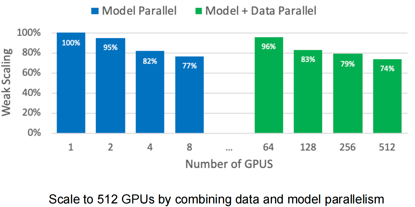
Achieves 74% weak scaling efficiency at 512 GPUs for an 8.3B parameter model.
Pipeline Model Parallelism
Motivation
Problem with naive model parallelism: Sequential execution leads to severe GPU under-utilization.
Consider a 4-layer model split across 4 GPUs:
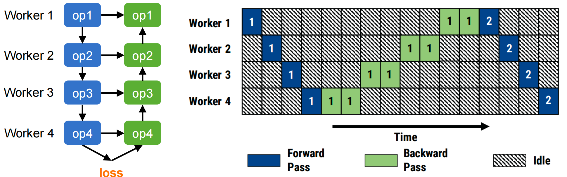
Only one GPU active at a time during forward pass, then again during backward. Utilization ≈ 25%!
Solution: Pipeline parallelism — process multiple micro-batches concurrently.
Basic Concept
Mini-batch: Total samples processed per training iteration (e.g., 32 samples)
Micro-batch: Subdivide mini-batch into smaller chunks (e.g., 4 micro-batches × 8 samples each)
Idea: While GPU 1 processes micro-batch 2, GPU 2 can process micro-batch 1, and so on.
GPipe Schedule
The original GPipe schedule completes all forward passes before starting backward:

Bubble time (idle periods):
\[ \text{BubbleFraction} = \frac{(p-1) \times (t_f + t_b)}{m \times t_f + m \times t_b} = \frac{p-1}{m} \]
where: - \(p\) = number of pipeline stages - \(m\) = number of micro-batches - \(t_f, t_b\) = time for forward/backward of one micro-batch
Problem: Must store activations for all \(m\) micro-batches until backward starts — high memory cost.
1F1B (One-Forward-One-Backward) Schedule
Improvement: Interleave forward and backward passes to free activation memory sooner.

Three phases: 1. Warm-up: Fill pipeline with forward passes (first \(p\) micro-batches) 2. Steady state: Alternate one forward and one backward (1F1B pattern) 3. Cool-down: Drain pipeline with remaining backward passes
Benefits: - Reduced memory: Only need to store activations for \(p\) micro-batches (pipeline depth) instead of \(m\) total micro-batches - Same bubble fraction: \(\frac{p-1}{m}\) (no performance degradation)
In-flight micro-batches: GPipe requires \(m\), 1F1B requires only \(p\) — typically \(p \ll m\).
Interleaved 1F1B Schedule
Further optimization: Divide each pipeline stage into \(v\) smaller sub-stages (chunks).
Each device is assigned \(v\) non-contiguous sub-stages instead of one contiguous stage.

Bubble time reduction: \[ \text{BubbleFraction}_{\text{interleaved}} = \frac{1}{v} \times \frac{p-1}{m} \]
Trade-off: - ✅ Bubble time reduced by factor of \(v\) (better GPU utilization) - ❌ Communication increased by factor of \(v\) (more frequent transfers between sub-stages)
When to use: When bubble time dominates and high-speed interconnect is available (e.g., NVLink, InfiniBand).
Pipeline Efficiency Analysis
Improving efficiency: Two knobs to reduce bubble fraction \(\frac{p-1}{m}\)
- Increase \(m\)
(more micro-batches):
- ✅ Reduces bubble time
- ❌ Caveat: Large total batch size may hurt convergence; small micro-batch size reduces GPU compute efficiency
- Decrease \(p\)
(fewer pipeline stages):
- ✅ Reduces bubble time
- ❌ Caveat: Increases per-stage memory requirement
Typical configuration: Choose \(m \geq 4p\) to achieve bubble fraction ≤ 25%.
Comparing Parallelization Strategies

Recommendation: Modern large-scale training combines all three approaches.
3D Parallelism: Combining All Strategies
DeepSpeed and similar frameworks implement 3D parallelism to train trillion-parameter models:

Three orthogonal dimensions:
- Data Parallelism: Across data-parallel groups (outer dimension)
- Tensor Model Parallelism: Within layers (e.g., 4-way split of attention/MLP)
- Pipeline Model Parallelism: Across layers (e.g., 4 pipeline stages)
Example: 800 GPUs = 64 data-parallel replicas × 2 tensor-parallel × 4 pipeline stages
Scaling results:
- 1 trillion parameters trainable on 800 A100 GPUs
- 30-40 TFLOPS/GPU sustained throughput
- Near-linear scaling up to hundreds of GPUs
Key to success:
- High-speed intra-node interconnect (NVLink) for tensor parallelism
- High-bandwidth inter-node network (InfiniBand) for data/pipeline parallelism
- Careful overlap of communication and computation
Interview Review Q&A
Part 1: Core Concepts (High-Frequency Interview Questions)
Q1: Explain the workflow of Data Parallelism. What does each GPU do during one training iteration? How are gradients synchronized?
In data parallelism, each mini-batch of data is distributed to different GPUs, where every GPU holds a full copy of the model parameters. Each GPU independently performs forward and backward passes to compute local gradients. The gradients are then synchronized across all GPUs via AllReduce, so every GPU obtains the same aggregated gradient. Finally, each GPU performs a local parameter update, keeping all model copies identical.
One iteration workflow:
- Forward: Each GPU computes predictions on its local mini-batch using the full model
- Backward: Each GPU computes gradients for all parameters based on its local loss
- Gradient Sync (AllReduce): Aggregate gradients across all GPUs so every GPU has the same result
- Local Weight Update: Each GPU independently applies the optimizer step with the aggregated gradient
Key invariant: All GPUs maintain identical parameters at all times (after each sync).
Q2: What are the main AllReduce implementations? Compare the total communication of Ring AllReduce vs. Naive AllReduce, and explain why Ring AllReduce is more scalable.
Main implementations: Naive AllReduce, Ring AllReduce, Tree AllReduce, Butterfly AllReduce.
Communication comparison (M = parameter size, N = number of workers):
| Algorithm | Total Communication | Per-Worker Communication |
|---|---|---|
| Naive AllReduce | \(N(N-1)M = O(N^2 M)\) | \((N-1)M\) |
| Ring AllReduce | \(2(N-1)M \approx 2NM\) | \(2 \cdot \frac{N-1}{N} \cdot M \approx 2M\) |
Why Ring AllReduce is more scalable:
- Per-worker communication is constant: Each worker sends/receives approximately \(2M\) regardless of N. Adding more GPUs does not increase any individual worker’s communication burden.
- Full bandwidth utilization: All links on the ring transmit data in parallel, maximizing aggregate bandwidth.
- No bottleneck node: Unlike parameter server or tree root, no single worker handles disproportionate traffic.
In contrast, Naive AllReduce has \(O(N)\) per-worker communication, which degrades linearly as workers are added.
Q3: In mixed-precision training with Adam optimizer, for a model with Ψ parameters, what does each GPU need to store and how much memory does each component take?
| Component | Precision | Size |
|---|---|---|
| FP16 Parameters | FP16 | \(2\Psi\) bytes |
| FP16 Gradients | FP16 | \(2\Psi\) bytes |
| FP32 Parameter Copy (master weights) | FP32 | \(4\Psi\) bytes |
| FP32 Gradient Copy | FP32 | \(4\Psi\) bytes |
| FP32 First Moment (momentum) | FP32 | \(4\Psi\) bytes |
| FP32 Second Moment (variance) | FP32 | \(4\Psi\) bytes |
| Total | \(20\Psi\) bytes |
Explanation:
- FP16 parameters and gradients (\(2\Psi + 2\Psi = 4\Psi\)): Used for the actual forward/backward computation (faster, less memory).
- FP32 optimizer states (\(4\Psi + 4\Psi + 4\Psi + 4\Psi = 16\Psi\)): The Adam optimizer requires FP32 precision for numerical stability. This includes the master weight copy, gradient copy, first moment (momentum), and second moment (variance).
This \(4\Psi + 16\Psi = 20\Psi\) decomposition is the foundation for understanding ZeRO Stage 1/2/3 memory partitioning.
Part 2: ZeRO Deep Dive
Q4: Explain ZeRO Stage 1/2/3 in your own words. What does each stage partition, and what does it keep replicated?
ZeRO Stage 1: Partitions optimizer states (FP32 parameter copy, momentum, variance, and FP32 gradient copy) across N GPUs. Each GPU stores only \(\frac{1}{N}\) of the optimizer states. Keeps replicated: full FP16 parameters and full FP16 gradients on every GPU.
ZeRO Stage 2: Builds on Stage 1 by additionally partitioning gradients. Each GPU stores only \(\frac{1}{N}\) of both optimizer states and gradients. Keeps replicated: full FP16 parameters on every GPU.
ZeRO Stage 3: Partitions everything — optimizer states, gradients, AND parameters. Each GPU stores only \(\frac{1}{N}\) of all model state. Nothing is replicated; parameters are gathered on-demand during forward/backward and discarded afterward.
Progressive partitioning summary:
| Stage | Partitioned | Replicated |
|---|---|---|
| ZeRO-1 | Optimizer states (\(16\Psi\)) | FP16 params (\(2\Psi\)) + FP16 grads (\(2\Psi\)) |
| ZeRO-2 | Optimizer states + Gradients (\(18\Psi\)) | FP16 params (\(2\Psi\)) |
| ZeRO-3 | Everything (\(20\Psi\)) | Nothing |
Q5: Walk through ZeRO Stage 1 during one complete training iteration. What happens during forward, backward, weight update, and parameter sync? What communication operations are involved?
Forward: Each GPU uses its local complete FP16 parameters to compute the forward pass normally. No communication needed.
Backward: Each GPU computes full FP16 gradients for all parameters on its local mini-batch. Then, an AllReduce is performed so every GPU obtains the same aggregated gradient across all workers.
Weight Update: Each GPU uses the aggregated gradient only for the partition it owns to update its local \(\frac{1}{N}\) of the optimizer states (apply Adam step). This produces updated FP16 parameter values for that partition only.
Parameter Sync: An AllGather operation collects the updated FP16 parameter partitions from all GPUs, so every GPU reconstructs the complete updated FP16 parameter set.
Communication operations: - AllReduce (gradient synchronization): \(\approx 2M\) communication - AllGather (parameter reassembly): \(\approx M\) communication
Q6: How does ZeRO Stage 2’s backward phase differ from Stage 1? Why can gradients be partitioned during the backward pass?
Stage 1: Performs a full AllReduce on gradients after backward is complete — every GPU ends up with the complete aggregated gradient.
Stage 2: Replaces AllReduce with Reduce-Scatter — each GPU only receives the aggregated gradient for its own partition. Gradients for other partitions are not stored.
Why gradients can be partitioned during backward:
Backward propagation proceeds layer by layer. Once all GPUs have computed the gradient for a given layer, the Reduce-Scatter for that layer can execute immediately — there is no need to wait for all layers to finish. After Reduce-Scatter completes for a layer, each GPU discards the gradient portions that belong to other GPUs’ partitions, freeing memory on the spot.
This is possible because each GPU only needs the gradients for the parameters it is responsible for updating. The layer-by-layer nature of backpropagation enables overlapping gradient computation with gradient communication, hiding latency.
Q7: ZeRO Stage 3 requires AllGather during both forward and backward to retrieve full parameters. Why is the total communication 1.5x baseline rather than 2x or 3x? Provide a quantitative analysis.
Baseline (standard data parallelism): One AllReduce per iteration = \(2M\) communication per worker (AllReduce = Reduce-Scatter + AllGather, each \(\approx M\)).
ZeRO Stage 3 per worker:
| Phase | Operation | Communication |
|---|---|---|
| Forward | AllGather parameters (gather before each layer, discard after) | \(M\) |
| Backward | AllGather parameters (need them again since discarded after forward) | \(M\) |
| Backward | Reduce-Scatter gradients (partition aggregated gradients) | \(M\) |
| Total | \(3M\) |
Ratio: \(\frac{3M}{2M} = 1.5\times\) baseline.
Why not 2x or 3x? - It is NOT 2x because the backward Reduce-Scatter replaces the baseline’s AllReduce — it’s the same gradient sync, just in partitioned form. - It is NOT 3x because the two AllGathers (forward + backward) each cost only \(M\), not \(2M\). Together they add \(2M\), replacing the baseline’s implicit parameter access (which had zero communication cost since parameters were replicated). - Net additional cost over baseline: \(+M\) (one extra AllGather for forward pass parameters), giving \(3M\) vs \(2M\) = 1.5x.
Part 3: Concrete Calculation — 7B Model Memory
Q8: Calculate the per-GPU memory for a 7B parameter model across all ZeRO stages with N = 64 GPUs.
Given: \(\Psi = 7\text{B}\), \(N = 64\)
Baseline (no partitioning): \[20 \times 7\text{B} = 140\text{ GB}\] This exceeds A100-80GB — baseline data parallelism cannot even load the model!
Detailed calculation for each stage:
| Stage | Formula | Calculation | Result |
|---|---|---|---|
| Baseline DP | \(20\Psi\) | \(20 \times 7\text{B}\) | 140 GB (OOM!) |
| ZeRO-1 | \(4\Psi + \frac{16\Psi}{N}\) | \(28\text{ GB} + 1.75\text{ GB}\) | 29.75 GB |
| ZeRO-2 | \(2\Psi + \frac{18\Psi}{N}\) | \(14\text{ GB} + 1.97\text{ GB}\) | 15.97 GB |
| ZeRO-3 | \(\frac{20\Psi}{N}\) | \(\frac{140}{64}\) | 2.19 GB |
Formula breakdown:
- Baseline: FP16 params (\(2\Psi\)) + FP16 grads (\(2\Psi\)) + FP32 optimizer states (\(16\Psi\)) = \(20\Psi\)
- ZeRO-1: FP16 params (\(2\Psi\)) + FP16 grads (\(2\Psi\)) + partitioned optimizer states (\(\frac{16\Psi}{N}\)) = \(4\Psi + \frac{16\Psi}{N}\)
- ZeRO-2: FP16 params (\(2\Psi\)) + partitioned grads (\(\frac{2\Psi}{N}\)) + partitioned optimizer states (\(\frac{16\Psi}{N}\)) = \(2\Psi + \frac{18\Psi}{N}\)
- ZeRO-3: Everything partitioned = \(\frac{(2+2+16)\Psi}{N} = \frac{20\Psi}{N}\)
Key interview takeaways:
- A 7B model with baseline DP cannot fit on a single A100-80GB — the 140 GB memory footprint is the dominant constraint
- ZeRO-1 brings it down to ~30 GB — comfortably fits on A100-80GB
- ZeRO-3 reduces model state to only ~2.2 GB — but note that activation memory is additional and can be substantial depending on batch size and sequence length
- The jump from baseline to ZeRO-1 provides the largest absolute savings (140 GB → 30 GB), while ZeRO-2 and ZeRO-3 provide further reductions at the cost of more communication complexity