
11868 LLM Sys: Decoding
Decoding: Sampling, Beam Search and Speculative Decoding
For foundational concepts (greedy decoding, beam search basics, sampling methods, KV cache, compute- vs memory-bound analysis), see my 11711 Advanced NLP: Decoding Algorithms notes. This post focuses on the systems-level details not covered there.
Efficient Discrete Sampling
At each decoding step, we need to sample from a categorical distribution over the vocabulary. This is a systems bottleneck worth optimizing.
Sampling Complexity
Given \(k\) categories with probabilities \(p_1, p_2, \ldots, p_k\), and \(n\) samples to draw:
| Method | Complexity | Notes |
|---|---|---|
| Direct sampling | \(O(nk)\) | Linear scan through CDF each time |
| Binary search | \(O(k + n \log k)\) | Build CDF once, binary search per sample |
| Alias sampling | \(O(k \log k + n)\) | Build alias table once, \(O(1)\) per sample |
Note on Alias Sampling: Alias sampling’s \(O(1)\)-per-sample advantage only pays off when drawing many samples from the same distribution (e.g., Monte Carlo simulations). In LLM decoding, the distribution changes at every step (\(n=1\) per distribution), so the alias table cannot be reused and must be rebuilt each time at \(O(k \log k)\) cost — offering no benefit. This motivates the Gumbel Max Trick below.
In PyTorch, the standard approach: 1
2probs = torch.softmax(logits, dim=-1)
next_token = torch.multinomial(probs, num_samples=1)
Gumbel Max Trick
A faster alternative that avoids computing softmax entirely.
Key theorem: Sampling from \(\text{Categorical}(\text{Softmax}(h))\) is equivalent to:
\[ x_i = h_i - \log(-\log(z_i)), \quad z_i \sim \text{Uniform}(0, 1) \] \[ \text{sampled token} = \arg\max_i \; x_i \]
Theory: \(x_i\) follows a Gumbel distribution, and \(\arg\max_i x_i\) follows \(\text{Categorical}\left(\frac{\exp(h_i)}{\sum_{j=1}^{k} \exp(h_j)}\right)\).
Why it’s useful: Replace softmax + multinomial sampling with addition + argmax, which is more hardware-friendly. The Gumbel noise can be pre-computed.
1 | class GumbelSampler: |
Reference: Kool et al. “Stochastic Beams and Where to Find Them: The Gumbel-Top-k Trick for Sampling Sequences Without Replacement.” ICML 2019.
Beam Search: Algorithm Details & Pruning
Beyond the basic beam search concept, this section covers the full algorithm implementation and pruning optimizations.
Algorithm Details
The full beam search procedure with a priority queue:
1 | best_scores = [] |
Key implementation details: - Use a min-heap priority queue of size \(k\) — always evict the lowest-scoring candidate - EOS-terminated sequences are kept but prevented from expanding (assign \(-\infty\) to all tokens except EOS) - Score is the cumulative log-probability (sum of log-probs)
Pruning Strategies
To reduce computation, candidates can be pruned early (Freitag & Al-Onaizan, 2017):
1. Relative Threshold Pruning
Given pruning threshold \(r_p\) and candidate set \(C\), discard candidate \(c\) if:
\[ \text{score}(c) \leq r_p \cdot \max_{c' \in C} \text{score}(c') \]
2. Absolute Threshold Pruning
Discard candidate \(c\) if:
\[ \text{score}(c) \leq \max_{c' \in C} \text{score}(c') - a_p \]
3. Relative Local Threshold Pruning
Apply thresholding per expansion step (local) rather than globally.
Combining Sampling and Beam Search
A hybrid approach: 1. Sample the first few tokens (introducing diversity) 2. Beam search for the remaining tokens (ensuring quality)
Why: Pure beam search tends to produce repetitive, low-diversity outputs. Sampling the initial tokens creates diverse prefixes, and beam search refines each prefix into a high-quality completion.
Code Example
Speculative Decoding: In Depth
Building on the basic speculative decoding concept, this section covers the validation mechanism, performance tradeoffs, and alignment considerations in detail.
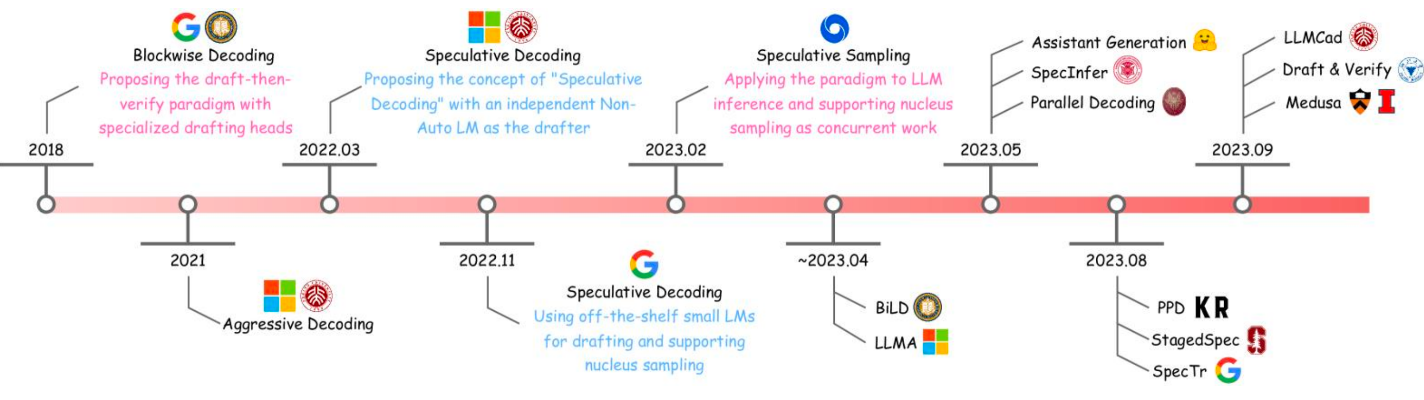
Recall the core flow: a small draft model \(f_{\text{draft}}\) generates \(N\) tokens \(y_{1:N} \sim f_{\text{draft}}(\cdot \mid x)\), then the large target model \(f_{\text{target}}\) validates them in a single forward pass.
Validation Criterion
Each draft token \(y_i\) is accepted if it appears in the target model’s top-\(K\) predictions:
\[ \text{Accept } y_i \quad \text{if} \quad y_i \in \text{TopK}\left(f_{\text{target}}(\cdot \mid x, y_{1:i-1})\right) \]
The target model computes \(f_{\text{target}}(\cdot \mid x, y_{1:i-1})\) for each prefix — but all of these are computed in the same forward pass because causal attention allows parallel likelihood computation for all prefix positions.
Rejection Handling
If a draft token \(y_i\) is rejected, the target model discards \(y_i\) and all subsequent draft tokens \(y_{i+1:N}\). The target model then generates from the last accepted position onward.
Worst case: All \(N\) tokens rejected → falls back to normal autoregressive decoding (no quality loss, just wasted draft computation).
Why is it Faster?
The key insight: validating \(N\) tokens is cheaper than generating \(N\) tokens.
- Generating \(N\) tokens: \(N\) sequential forward passes through the target model
- Validating \(N\) tokens: 1 forward pass through the target model (causal attention computes likelihoods for all positions simultaneously)
The draft model’s forward passes are cheap (small model). So the total cost is roughly: \(N\) cheap draft passes + 1 expensive target pass, vs. \(N\) expensive target passes.
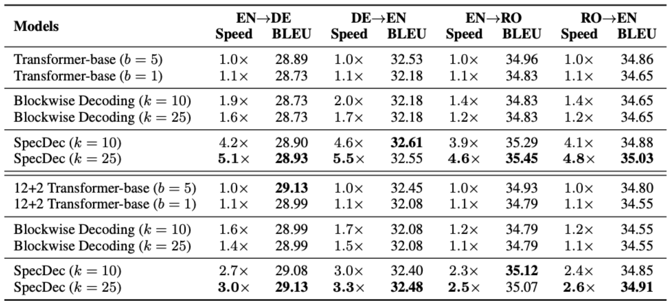
Choosing \(N\) (Draft Length)
| Large \(N\) | Small \(N\) |
|---|---|
| ✅ Higher theoretical speedup | ✅ Lower rejection cost |
| ❌ Higher chance of rejection | ❌ Less parallelism benefit |
| ❌ More softmax computations (memory pressure) | ✅ Lower memory overhead |
| ❌ Longer stall times for real-time applications | ✅ Better for interactive use |
Popular choices: \(N = 4\) or \(N = 8\).
Alignment Considerations
The draft-target alignment (how well the draft model approximates the target) is critical: - Good alignment → low rejection rate → high speedup - Poor alignment → frequent rejections → speedup cancelled
Best practice: Choose draft and target models from the same model family (e.g., LLaMA-7B drafting for LLaMA-70B).
Empirical Results
Speculative decoding has been shown to: - Generate text of comparable quality to standard autoregressive decoding - Achieve significant wall-clock speedups (typically 2-3x) depending on draft-target alignment
EAGLE: Extrapolation Algorithm for Greater Language-model Efficiency
EAGLE improves upon vanilla speculative decoding with a key observation: the next token’s final-layer feature is easier to predict than the next token itself.
Motivation
Vanilla speculative decoding uses a separate small LM as the draft model, which predicts the next token. But predicting a discrete token from the full vocabulary is hard. EAGLE instead predicts the next final-layer feature vector using a single Transformer layer, then applies the original model’s LM head to get token predictions.
Architecture
EAGLE reuses two components from the original LLM: - The embedding layer (token → vector) - The LM head (feature → logits)
It adds one small Transformer layer that takes as input: - The concatenation of the token embedding \(e_t\) and the final-layer feature \(f_t\) from the target model
And outputs a predicted feature \(\hat{f}_{t+1}\), from which the LM head produces token predictions.
Why embedding + feature? The sampled token strongly affects the final-layer feature. For example, after “I am”, the features for “excited” vs. “begin” are very different. The token embedding captures this discrete choice, while the final-layer feature captures the contextual representation.

Tree-Structured Drafting
Instead of a single linear chain of draft tokens, EAGLE generates a tree of candidate continuations:
1 | "How can" |
Implementation uses tree attention: flatten all candidates into a single sequence with a tree-shaped attention mask, allowing efficient parallel computation.
Training
EAGLE’s draft layer is trained with a combined loss:
\[ L = L_{\text{reg}} + w_{\text{cls}} \cdot L_{\text{cls}} \]
Regression loss (feature prediction): \[ L_{\text{reg}} = \text{SmoothL1}\left(f_{i+1}, \; \text{DraftModel}(T_{2:i+1}, F_{1:i})\right) \]
where \(T_{2:i+1}\) are token embeddings and \(F_{1:i} = (f_1, \ldots, f_i)\) are target model features.
Classification loss (token prediction): \[ L_{\text{cls}} = \text{CrossEntropy}\left(p_{i+2}, \; \hat{p}_{i+2}\right) \]
where \(p_{i+2} = \text{Softmax}(\text{LMHead}(f_{i+1}))\) and \(\hat{p}_{i+2} = \text{Softmax}(\text{LMHead}(\hat{f}_{i+1}))\).
Results
EAGLE achieves significantly faster decoding than vanilla speculative decoding on MT-Bench, with minimal quality degradation.
Further Improvements
- EAGLE-2: Prunes low-confidence tokens in the draft tree, reducing wasted computation
- EAGLE-3: Scales the method to larger training datasets for better draft quality
Code
Summary
| Method | Type | Key Idea |
|---|---|---|
| Gumbel Max Trick | Efficient sampling | Replace softmax + multinomial with addition + argmax |
| Beam Search Pruning | Search optimization | Discard low-scoring candidates early |
| Speculative Decoding | Acceleration | Draft cheap, validate in parallel |
| EAGLE | Improved speculation | Predict features instead of tokens, tree-structured drafts |
Key takeaway: From a systems perspective, the bottleneck of LLM decoding is the sequential, memory-bound nature of autoregressive generation. Speculative decoding and EAGLE address this by converting serial generation into parallel validation — the fundamental insight being that verification is cheaper than generation with causal attention.
References
- Freitag & Al-Onaizan. “Beam Search Strategies for Neural Machine Translation.” 2017.
- Kool et al. “Stochastic Beams and Where to Find Them: The Gumbel-Top-k Trick for Sampling Sequences Without Replacement.” ICML 2019.
- Leviathan et al. “Fast Inference from Transformers via Speculative Decoding.” ICML 2023.
- Li et al. “EAGLE: Speculative Sampling Requires Rethinking Feature Uncertainty.” ICML 2024.
This post is based on lecture materials from CMU 11-868 LLM Systems by Lei Li.

