Transformer, Attention, and Optimizations

Course: 15-442/15-642 Machine Learning Systems Instructors: Tianqi Chen and Zhihao Jia Carnegie Mellon University

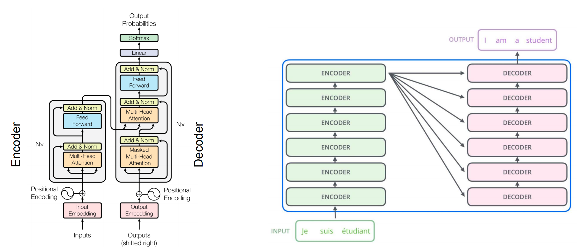
Attention Mechanism

The attention mechanism is an approach where individual states are combined using weights.

Basic Concept

For hidden states \(h_1, h_2, h_3, h_4\) from previous layer inputs \(x_1, x_2, x_3, x_4\):

\[ h_t = \sum_{i=1}^{t} s_i x_t \]

where \(s_i\) is the “attention score” that computes how relevant position \(i\)’s input is to the current hidden output.

Self-Attention

Self-attention maps a query and a set of key-value pairs to an output.

Mathematical Formulation

\[ A(Q, K, V) = \text{softmax}\left(\frac{QK^T}{\sqrt{d}}\right)V \]

Where: - Q (Query): \(N \times d\) matrix - K (Keys): \(N \times d\) matrix - V (Values): \(N \times d\) matrix - d: dimension of key/query/value vectors - N: sequence length

Computation Steps

Compute queries, keys, and values from input embeddings:
- \(Q = X W^Q\)
- \(K = X W^K\)
- \(V = X W^V\)
Calculate attention scores: \(S = QK^T\) (size: \(N \times N\))
Scale by \(\sqrt{d}\): \(S' = S / \sqrt{d}\)
Apply softmax: \(A = \text{softmax}(S')\)
Multiply by values: \(O = AV\)

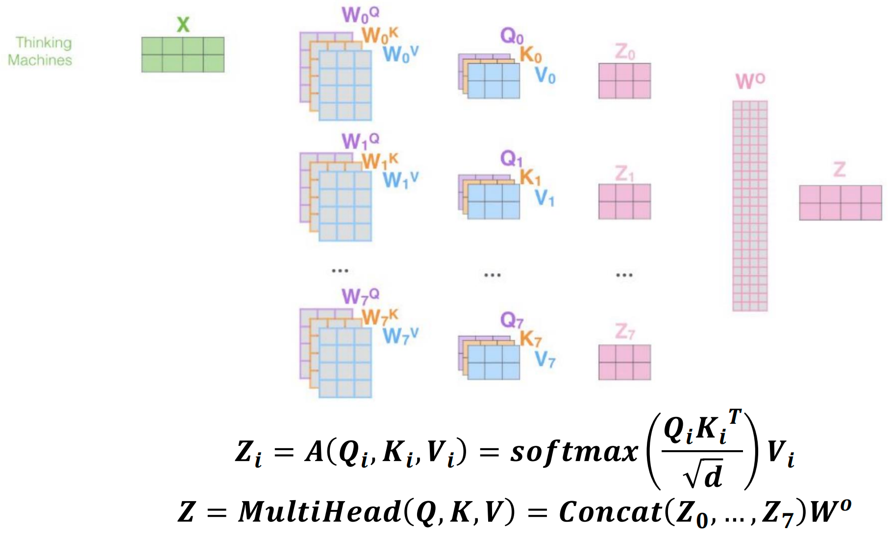
Multi-Head Self-Attention

Multi-head attention parallelizes attention layers with different linear transformations on input and output.

Benefits

More parallelism: Can process multiple representation subspaces simultaneously
Reduced computation cost per head: Each head works with smaller dimensions

Formulation

For each head \(i\): \[ Z_i = A(Q_i, K_i, V_i) = \text{softmax}\left(\frac{Q_i K_i^T}{\sqrt{d}}\right)V_i \]

Final output: \[ Z = \text{MultiHead}(Q, K, V) = \text{Concat}(Z_0, \ldots, Z_7)W^O \]

where typically 8 heads are used, each processing a \(d/8\) dimensional subspace.

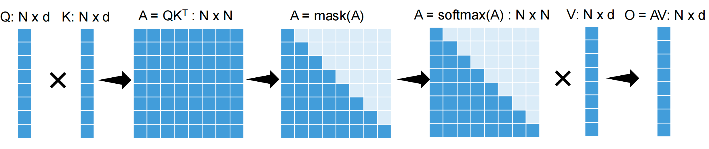
Computing Attention on GPUs - Challenges

Standard Attention Computation

The naive approach: \(O = \text{Softmax}(QK^T)V\)

Workflow: 1. \(A = QK^T\) : \(N \times N\) matrix 2. \(A = \text{mask}(A)\) (for causal attention) 3. \(A = \text{softmax}(A)\) : \(N \times N\) matrix 4. \(O = AV\) : \(N \times d\) matrix

Key Challenges

Large intermediate results: \(O(N^2)\) attention matrix
Repeated reads/writes from GPU device memory: Memory bandwidth bottleneck
Cannot scale to long sequences: Quadratic memory requirement

GPU Memory Hierarchy

NVIDIA A100 GPU:

Per-block shared memory (SRAM): 19 TB/s bandwidth, 20 MB capacity
- Readable/writable by all threads in a block
- Fast but small
Device global memory (HBM - High Bandwidth Memory): 1.5 TB/s bandwidth, 80 GB capacity
- Readable/writable by all threads
- ~12.6x slower than SRAM
- Large capacity but slower access

HBM (High Bandwidth Memory) is the GPU’s main memory - it has large capacity but is much slower than on-chip SRAM. FlashAttention’s core optimization is to minimize HBM accesses by doing as much computation as possible in fast SRAM.

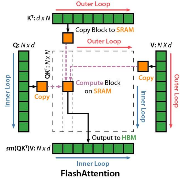
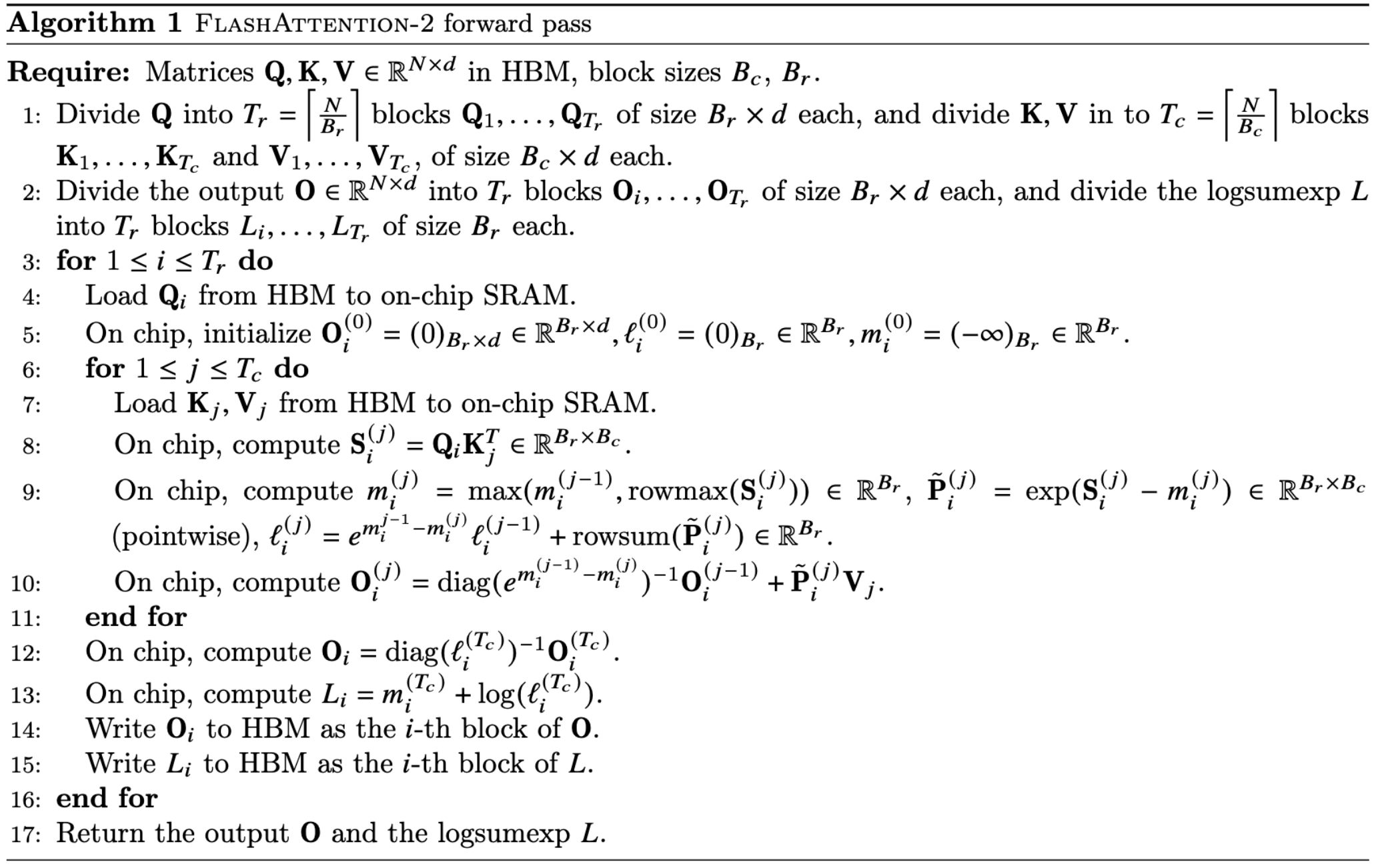
FlashAttention: IO-Aware Exact Attention

Key Idea

Compute attention by blocks to reduce global memory access

Two Main Techniques

1. Tiling

Restructure algorithm to load query/key/value block by block from global to shared memory:

Load inputs by blocks from HBM to SRAM
On-chip, compute attention output w.r.t. the block
Update output in device memory by scaling

2. Recomputation

Don’t store attention matrix from forward pass, recompute it in backward pass

Tradeoff: Increases FLOPs but reduces memory I/O

In the GPU, the bandwidth is the bottleneck

Metric	Standard	FlashAttention
GFLOPs	66.6	75.2 (+13%)
Global mem access	40.3 GB	4.4 GB (-89%)
Runtime	41.7 ms	7.3 ms (5.7x faster)

Safe Softmax and Online Softmax

Problem: Maximum value for 16-bit floating point is 65504 (< \(e^{12}\))

Solution: Compute softmax of vector \(x\) as:

\[ m(x) := \max_i x_i \] \[ f(x) := [e^{x_1-m(x)}, \ldots, e^{x_n-m(x)}] \] \[ \ell(x) := \sum_i f(x)_i \] \[ \text{softmax}(x) := \frac{f(x)}{\ell(x)} \]

For two vectors \(x^{(1)}\) and \(x^{(2)}\):

\[ m(x) = m([x^{(1)} \, x^{(2)}]) = \max(m(x^{(1)}), m(x^{(2)})) \]

\[ f(x) = [e^{m(x^{(1)})-m(x)} f(x^{(1)}), \, e^{m(x^{(2)})-m(x)} f(x^{(2)})] \]

\[ \ell(x) = e^{m(x^{(1)})-m(x)} \ell(x^{(1)}) + e^{m(x^{(2)})-m(x)} \ell(x^{(2)}) \]

FlashAttention-2 Algorithm

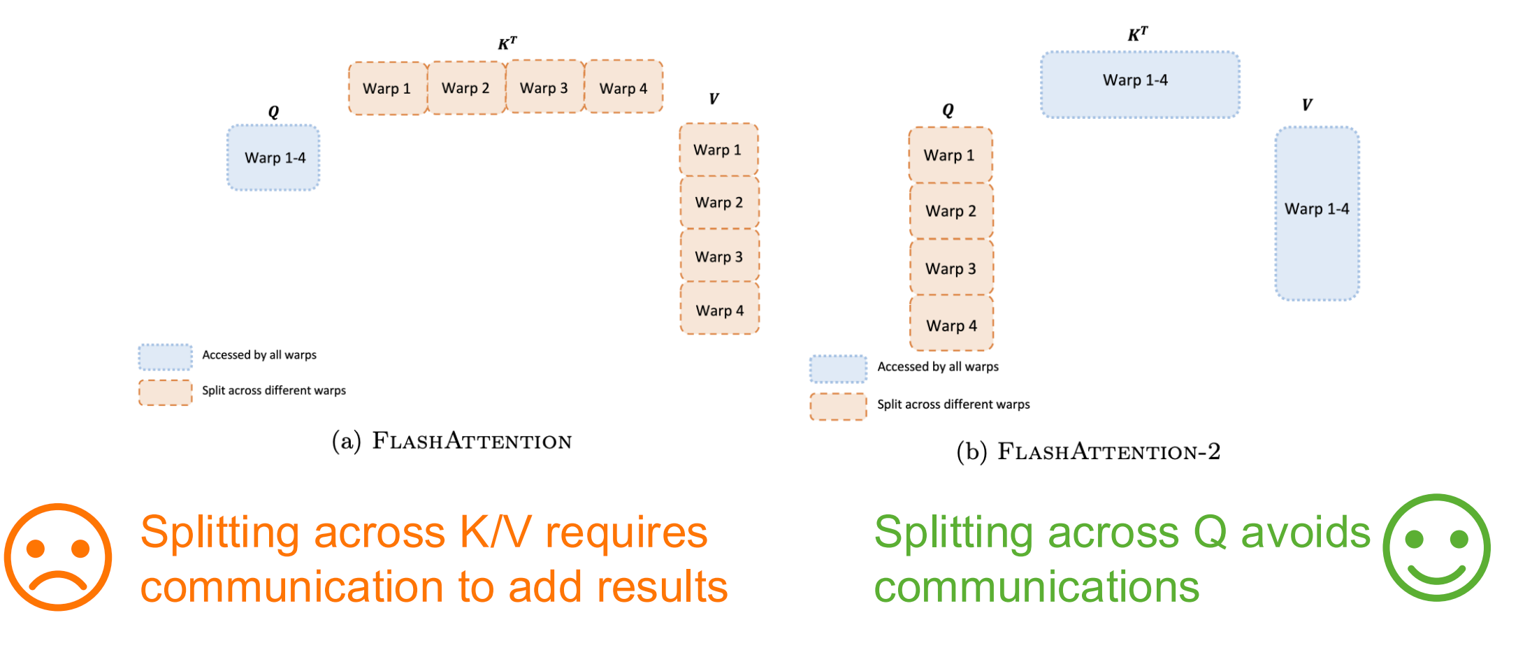
Parallelization Strategy

Thread Block Level: - Step 1: Assign different heads to different thread blocks (16-64 heads) - Step 2: Assign different queries to different thread blocks - Why not partition keys/values? Thread blocks cannot communicate; cannot perform softmax when partitioning keys/values

Warp Level: - FlashAttention: Split across K/V requires communication to add results ❌ - FlashAttention-2: Split across Q avoids communication ✅

Why Different Parallelization for Forward vs Backward Pass?

Forward Pass (Parallelize by Rows/Queries): - Computing \(O = \text{softmax}(QK^T)V\) - Each thread block processes different query rows independently - No communication needed - different rows are completely independent - Like students working on different problems independently

Backward Pass (Parallelize by Columns/Keys-Values): - Computing gradients requires updating \(dQ\): \[dQ_i = dQ_i + dS^{(j)} K_j\] - This update requires accumulation across different K/V blocks - Each column block contributes to the same \(dQ\) row - Requires atomic operations through HBM to coordinate updates - Like students working on different parts of the same problem - results must be combined

Key Difference: Forward pass has independent row computations, but backward pass needs to accumulate contributions from different blocks, requiring synchronization through HBM with atomic adds.

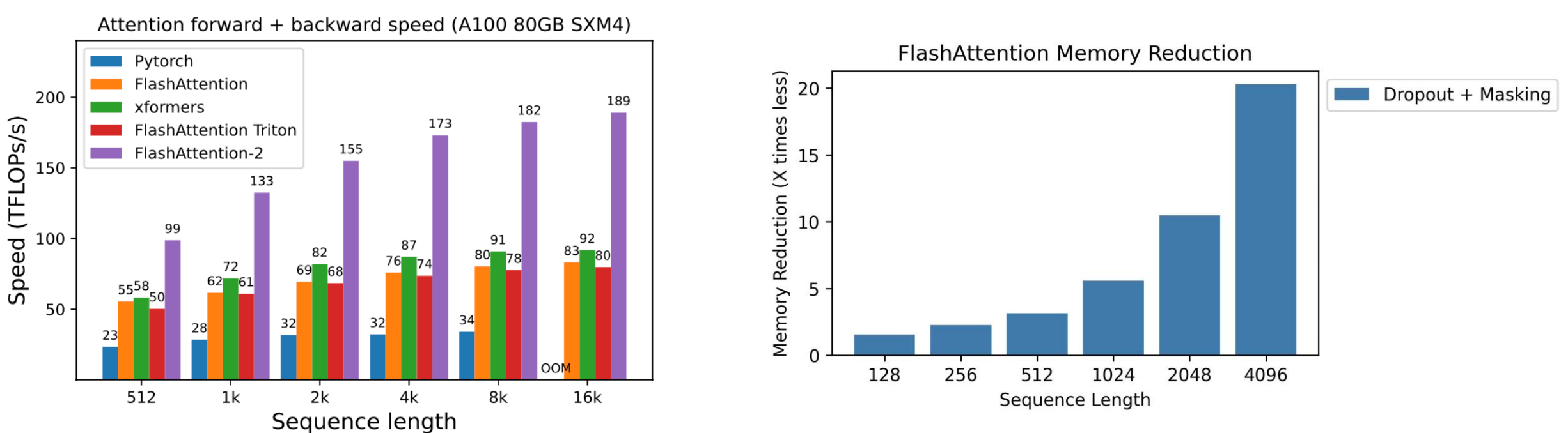
Performance

FlashAttention achieves: - 2-4x speedup over PyTorch and other baselines - 10-20x memory reduction - Linear memory scaling with sequence length (vs quadratic)

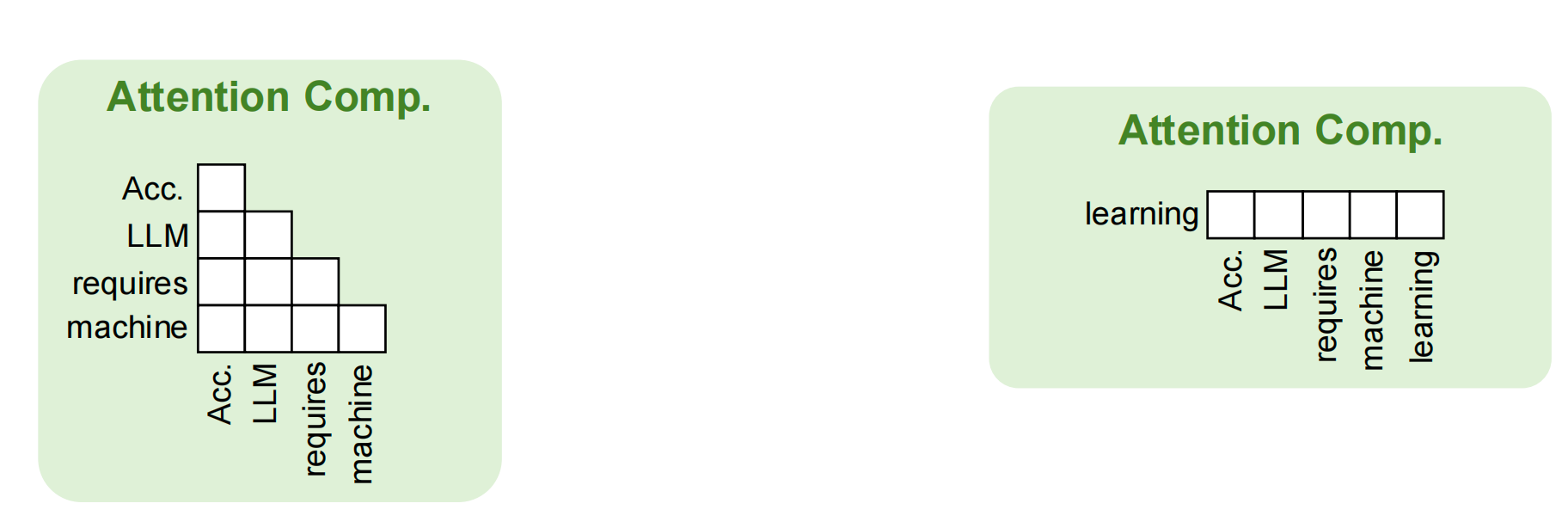
Generative LLM Inference: Autoregressive Decoding

Two Phases

1. Pre-filling Phase (Iteration 0)

Process all input tokens at once
Compute attention for entire prompt
Example: [Accelerating LLM requires machine] → output: learning

2. Decoding Phase (Iterations 1+)

Process a single token generated from previous iteration
Use attention keys & values of all previous tokens
Example iterations:
- Iter 1: learning → systems
- Iter 2: systems → optimizations
- Iter 3: optimizations → [EOS]

Key-Value Cache

Purpose: Save attention keys and values for following iterations to avoid recomputation

Memory: Grows linearly with sequence length

Attention computation in decoding:

Query: single new token
Keys/Values: all previous tokens (from cache)

FlashAttention for LLM Inference

Applicability

Pre-filling phase: ✅ Yes - Can compute different queries using different thread blocks/warps

Decoding phase: ❌ No - There is only a single query in the decoding phase - FlashAttention processes K/V sequentially - Inefficient for requests with long context (many keys/values)

Flash-Decoding: Parallel Attention for Decoding

Key Insight

Attention is associative and commutative - can be split and reduced

Approach

Split keys/values into small chunks
Compute attention with these splits using FlashAttention (in parallel)
Reduce results across all splits

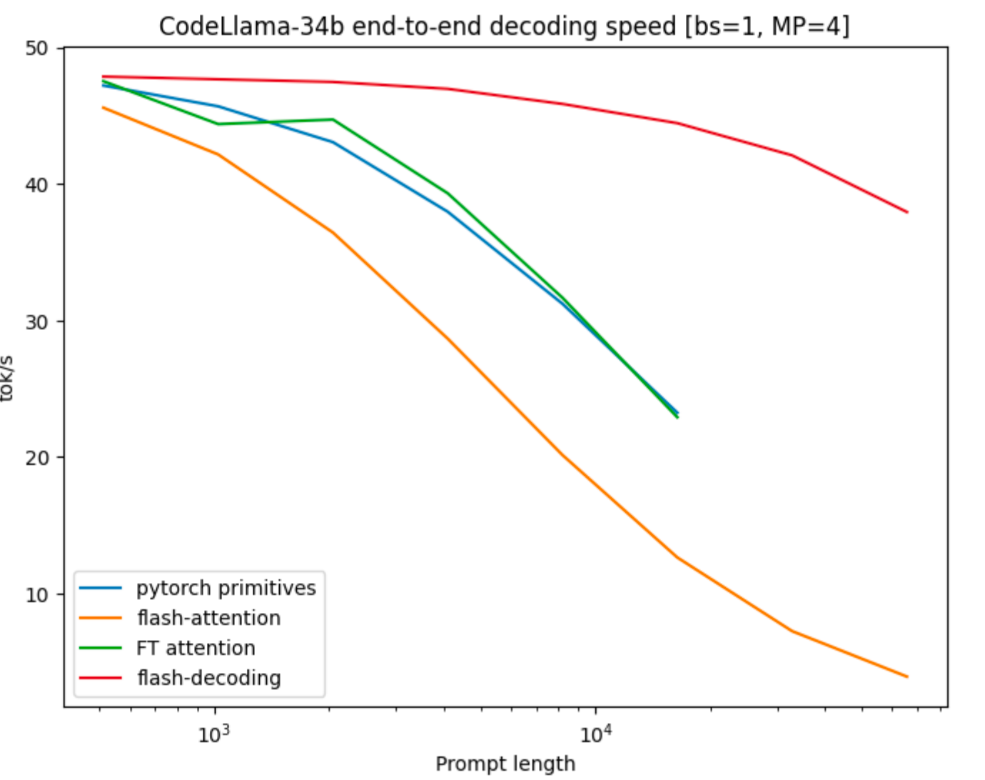
Performance

Flash-Decoding is up to 8x faster than prior work for long contexts

Example (CodeLlama-34b, bs=1, MP=4): - Sequence length 1K: ~47 tok/s (similar to others) - Sequence length 16K: ~38 tok/s vs ~5 tok/s (FlashAttention) - Maintains high throughput even for very long sequences

Summary

Attention mechanism is core to Transformer models, with \(O(N^2)\) complexity
Multi-head attention provides parallelism and representation diversity
FlashAttention uses tiling and recomputation to achieve IO-efficiency:
- 2-4x speedup, 10-20x memory reduction
- Enables longer sequence lengths
LLM inference has two phases with different computation patterns:
- Pre-filling: many queries (batched)
- Decoding: single query (sequential)
Flash-Decoding parallelizes across keys/values for efficient long-context decoding:
- Up to 8x faster for long sequences
- Critical for applications requiring large context windows