Lec6 Pretraining

Basic Idea

The pretrained base model will be adapted to downstream tasks.

Transfer learning: take “knowledge” from one task and apply it to another task

• Less task data: use less data to reach a given level of performance

• Better task performance: reach higher performance than training from scratch

• One model, multiple tasks: convenient, amortizes cost, a starting point for many uses, …

Major Factors

Each model is influenced by 4 major factors:

• Architecture: neural network architecture

• Task: what the model predicts (e.g. next-token)

• Data: the data used to train the model

• Hyper-parameters: e.g. learning rate, batch size

Masked Language Modeling

Masked Language Modeling (MLM) trains a language model to predict masked tokens given the remaining visible context. This objective is widely used in bidirectional models such as BERT.

The MLM loss is defined as:

\[ \mathcal{L}_{\text{MLM}}(\theta; D) = -\frac{1}{|D|} \sum_{x \in D} \;\mathbb{E}_{M \sim \text{corrupt}(x)} \sum_{t \in M} \log p_\theta(x_t \mid x_{-M}) \]

\(x \in D\): an input sequence (sentence) from the dataset
\(M\): a randomly sampled set of masked token positions
\(\text{corrupt}(x)\): the masking (corruption) process applied to \(x\)
\(x_{-M}\): all unmasked tokens in the sequence
\(x_t\): the ground-truth token at position \(t\)
\(p_\theta(x_t \mid x_{-M})\): model probability of predicting \(x_t\) given the visible context
Denoising Perspective MLM can be viewed as a denoising autoencoder: the input is corrupted by masking tokens, and the model learns to reconstruct the original sequence.
Pseudo-likelihood Objective: Instead of modeling the full joint likelihood of the sequence, MLM maximizes the sum of conditional log-probabilities of masked tokens given the rest of the sequence. This corresponds to maximizing a pseudo-likelihood rather than a true joint likelihood.

Autoregressive Language Modeling

Predict the next token (x_t) given all previous tokens (x_{<t}). [ {}(; D) = - {x D} {t=1}^{|x|} p(x_t x_{<t}) ] Key Properties - Maximizes the likelihood of the training data
- Fits the true data distribution (p_)
- Equivalent to cross-entropy with a one-hot target distribution
- Can be interpreted as learning to compress data generated by (p_)

Evaluate a model

Loss(traning, validation, test)
- Diagnose training trajectory, compare models in the same family
Few-shot prompting
Fine-tuning

Data

Quantity: How much data do I have?
Quality: Is it beneficial for training? (Extraction, Filtering, Deduplication)
Coverage: Does the data cover the domain(s) I care about, and in the right proportions?
- We can train a classifier filtering to help us detect the content

Lec7 Scaling Laws and In-Context Learning

Scaling Laws

Training = Spending Compute

Given a fixed pretraining budget, how should we allocate the budget to achieve the best possible model?

Core approximation for transformer LMs (Kaplan et al. 2020): \[ C \approx 6ND \]

N = number of parameters, D = number of tokens, C = FLOPs
Example: Llama 2 7B on 2T tokens → C ≈ 8.4 × 10²² FLOPs

Central question: Given fixed C, how to split between N and D?

Power Laws

\[ L = a \cdot x^{b} \quad \Rightarrow \quad \log L = \log a + b \cdot \log x \]

Doubling x → L becomes L · 2ᵇ. With b = −0.095, doubling data only reduces loss by ~6.4%. Diminishing returns are severe — exponentially more resources for linear loss improvement.

Data Scaling

\[ L = (D / D_c)^{-b} \]

Three regions: small data → power-law region → irreducible error (bounded by data entropy)
Repeated data: ~4 epochs ≈ new data; ~40 epochs → worthless (Muennighoff+ 2025)
Different domains (Wikipedia, Books, Common Crawl) have different scaling curves

Model Size Scaling

\[ L = (N / N_c)^{-b} \]

Larger models are more sample-efficient (reach lower loss with fewer tokens)
Transformers scale significantly better than LSTMs

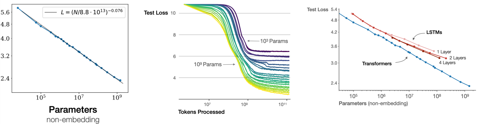
Compute-Optimal Training

Paper	N_opt	D_opt	Implication
Kaplan et al. 2020	∝ C⁰·⁷³	∝ C⁰·²⁷	Prioritize bigger models
Chinchilla (Hoffmann et al. 2022)	∝ C⁰·⁵	∝ C⁰·⁵	Scale N and D equally

∝ means proportional to

Chinchilla’s insight: many existing LLMs (e.g., Gopher 280B) were undertrained. This directly influenced LLaMA’s design — smaller models trained on much more data.

Run small-scale experiments → fit scaling laws → extrapolate optimal hyperparameters (model size, tokens, batch size, learning rate) for the expensive target run.

Prompting and In-Context Learning

Three Prompting Strategies

Strategy	Format	Key Issue
No prompt	Raw text completion	Uncontrollable
Zero-shot	Instruction + input	Output format unstable; wording-sensitive
Few-shot (ICL)	Instruction + K examples + input	Examples define format & task; no param updates

ICL Phenomena (Agarwal et al. 2024)

Task retrieval: sometimes input-only examples work as well as (input, output) pairs — ICL partly “retrieves” pretraining patterns rather than learning new mappings

Pretraining bias: default labels need few shots; flipped/abstract labels need many more to overcome built-in associations
Sensitivity: example ordering, label balance, and label coverage all significantly affect performance (Lu et al. 2021; Zhang et al. 2022)
Model variation: ability to benefit from many-shot varies greatly (Gemini 1.5 Pro improves up to 1024-shot; GPT-4-Turbo plateaus early)

Chat Prompts

Messages format with system / user / assistant roles → tokenizer converts to string with special tokens. System prompts define model behavior (reasoning strategy, safety rules, output format, etc.).

Chain-of-Thought (CoT)

Few-shot CoT (Wei et al. 2022): include reasoning steps in examples
Zero-shot CoT (Kojima et al. 2022): append “Let’s think step by step”
Key insight: CoT gives the model adaptive computation time — each reasoning token is an extra forward pass

Prompt Chains

Chain multiple LLM calls (with different prompts / external tools) sequentially:

1	input → LLM₁ → intermediate → LLM₂ → intermediate → ... → output

Enables problem decomposition, tool use (search, code execution), and multi-step reasoning.

Lec8 Fine-Tuning

What is Fine-Tuning?

Continued gradient-based training of a pre-trained model on task-specific data. Given pre-trained parameters θ₀ and dataset D = {(x, y)ₙ}: \[ \theta^* = \arg\min_\theta \mathbb{E}_{(x,y)\sim D} [\mathcal{L}(f_\theta(x), y)] \] Also called Supervised Fine-Tuning (SFT). Use regularization/dropout to prevent overfitting.

Two Fine-Tuning Paradigms

Classification fine-tuning: Add a linear head on the last hidden state. \[ p_\theta(y \mid x) = \text{softmax}(Wh + b), \quad W \in \mathbb{R}^{K \times d}, \; b \in \mathbb{R}^K \]

Loss: cross-entropy \(\mathcal{L} = -\log p_\theta(y \mid x)\)
Update all parameters \(\theta = (\theta_0, W, b)\)

Language model fine-tuning: Keep the LM architecture, train on (input, output) pairs.

Keep the LM architecture, train on (input, output) pairs. Concatenate as [start] x [sep] y [end], compute loss only on output tokens:

\[ \mathcal{L}_{\text{MLE}} = -\sum_{t=1}^{T} \log p_\theta(y_t \mid x, y_{<t}) \] No additional head needed — uses the existing LM head.

Which Parameters to Update?

Option	What’s Updated	Cost	Trade-off
Head only	\(K \times d + K\) params	Cheapest	Assumes pre-trained representations are already linearly separable
Full fine-tuning	All	\(\theta\)	May lead to overfitting
PEFT	Small subset	\(\theta\)	Can change the representations

LoRA (Low-Rank Adaptation) [Hu et al. 2021]

Key idea: approximate weight updates with low-rank matrices.

For weight \(W_0 \in \mathbb{R}^{d \times d'}\), decompose the update as:

\[ \Delta W = BA, \quad B \in \mathbb{R}^{d \times r}, \; A \in \mathbb{R}^{r \times d'}, \; r \ll \min(d, d') \]

Freeze \(W_0\), only train \(A\) and \(B\)
Final weight: \(W = W_0 + \frac{\alpha}{r} \cdot BA\)
Typically applied to \(W_q\) and \(W_v\) in attention layers
After training, merge \(\Delta W\) into \(W_0\) → no extra inference cost

Effects of Fine-Tuning

Data efficiency: Pre-trained models reach good performance with far fewer examples than training from scratch (Howard & Ruder 2018 — ULMFiT).

Distribution narrowing: Fine-tuning minimizes \(D_{\text{KL}}(p_{\text{finetune}} \| p_\theta)\) instead of \(D_{\text{KL}}(p_{\text{data}} \| p_\theta)\). The model’s distribution becomes narrower and specialized.

Side effects:

Summarization model fails at translation (lost generality)
Model becomes dependent on exact prompt formatting used during training
Few-shot learning ability may degrade after fine-tunin

Instruction Tuning

Fine-tune a model on (instruction + input, output) pairs across multiple tasks, so it learns to follow instructions generically.

Chat Tuning

Chat is just instruction tuning with conversational format:

System prompt + [user, assistant, user, assistant, …]
Special tokens mark role boundaries (e.g., <|start_header_id|>user<|end_header_id|>)
Instruction + input are implicitly embedded in the conversation

Data sources: OpenOrca (16 hand-written system prompts, GPT-4 outputs, 2.9M examples), LMSys-1M (real user conversations from online LLM service)

Knowledge Distillation

Use a strong teacher model to train a smaller student model. Both approaches minimize \(D_{\text{KL}}(q \| p_\theta)\) between teacher \(q\) and student \(p_\theta\).

Token-Level Distillation [Hinton et al. 2015]

Student mimics teacher’s full probability distribution at each token position:

\[ \mathcal{L}_{\text{distill}} = -\sum_{y_t \in V} q(y_t \mid y_{<t}, x) \cdot \log p_\theta(y_t \mid y_{<t}, x) \]

Uses soft labels (teacher’s distribution) instead of hard one-hot labels
Requires access to teacher’s logits
Richer signal than standard cross-entropy (which only uses the correct token)

Sequence-Level Distillation [Kim & Rush 2016]

Teacher generates complete outputs; student fine-tunes on them:

\[ \mathcal{L}_{\text{seq}} = \mathbb{E}_{y \sim q(y|x)} \left[-\log p_\theta(y \mid x)\right] \]

Only needs teacher’s generated text, not logits (black-box friendly)
Example: DeepSeek-R1-Distill-Qwen-7B = Qwen-7B fine-tuned on DeepSeek-R1’s outputs
Mathematically also minimizes \(D_{\text{KL}}(q \| p_\theta)\), just with Monte Carlo approximation

Augmented Teacher [West et al. 2022]

Teacher can be an augmented LLM:

\[ q \propto p_{\text{LLM}}(y \mid x) \cdot A(x, y) \] where \(A\) is a classifier/verifier. If the augmented teacher is better than \(p_{\text{LLM}}\) alone, the distilled student can surpass \(p_{\text{LLM}}\) — the student becomes better than its base teacher through filtered/verified data.

Lec9 Decoding Algorithms

Basic Setup

Autoregressive Language Model

\[ p_\theta(y_{1:T} | x) = \prod_{t=1}^{T} p_\theta(y_t | y_{<t}, x) \]

Next-Token Distribution

Each term \(p_\theta(y_t | y_{<t}, x)\) gives us a probability distribution over next tokens.

Decoding: Choose next tokens so that we end up with an output \(y_{1:T}\).

Decoding as Optimization

Goal: MAP Decoding

Find the most likely output: \[ \hat{y} = \arg\max_{y \in \mathcal{Y}} p_\theta(y | x) \]

Also called mode-seeking or maximum a-posteriori (MAP)
Key challenge: output space \(\mathcal{Y}\) is very large

Approach 1: Greedy Decoding

For \(t = 1 \ldots \text{End}\): \[ \hat{y}_t = \arg\max_{y_t \in V} p_\theta(y_t | \hat{y}_{<t}, x) \]

Limitation: Does not guarantee the most-likely sequence.

Approach 2: Beam Search

Width-limited breadth-first search
Maintain \(B\) likely paths at each step
\(B = 1\): greedy decoding
\(B = |V|^{T_{\max}}\): exact MAP (intractable)
In practice: \(B = 16\) (hyperparameter)

HuggingFace interface:

# Greedy
model.generate(do_sample=False, num_beams=1)

# Beam search
model.generate(do_sample=False, num_beams=16)

Pitfalls of MAP Decoding

1. Degeneracy - Repetition traps: Models assign high probability to repetitive loops - Short sequences: Highest-probability sequence might be empty - Remedy: length normalization

2. Atypicality - Most likely outcome ≠ typical outcome - Example: Biased coin \(\Pr[H] = 0.6\), most likely outcome of 100 flips is all heads (atypical!)

3. Probability spread - When multiple ways exist to express the same thing, probability spreads across variants - Highest-probability output may not be the “best”

Sampling

Ancestral Sampling

For \(t = 1 \ldots \text{End}\): \[ \hat{y}_t \sim p_\theta(y_t | \hat{y}_{<t}, x) \]

Equivalent to sequence sampling: \(y_{1:T} \sim p_\theta(y_{1:T} | x)\)
Implemented via categorical sampling (PyTorch, etc.)

HuggingFace interface:

1	model.generate(do_sample=True)

Problems with Ancestral Sampling

Heavy tail problem:

Even if each bad token has small probability, sum of bad tokens has nontrivial probability
Leads to incoherence

Compounding error: - Probability of sampling no bad tokens: \((1 - \epsilon)^T\) - Example: \(\epsilon = 0.01, T = 128 \Rightarrow p(\text{no bad tokens}) = 0.276\)

Workaround: Truncate the Tail

Top-k Sampling: Sample only from \(k\) most-probable tokens \[ \hat{y}_t \sim \begin{cases} p_\theta(y_t | y_{<t}, x) / Z_t & \text{if } y_t \text{ in top-}k \\ 0 & \text{otherwise} \end{cases} \]

Top-p Sampling: Sample only from top \(p\) probability mass

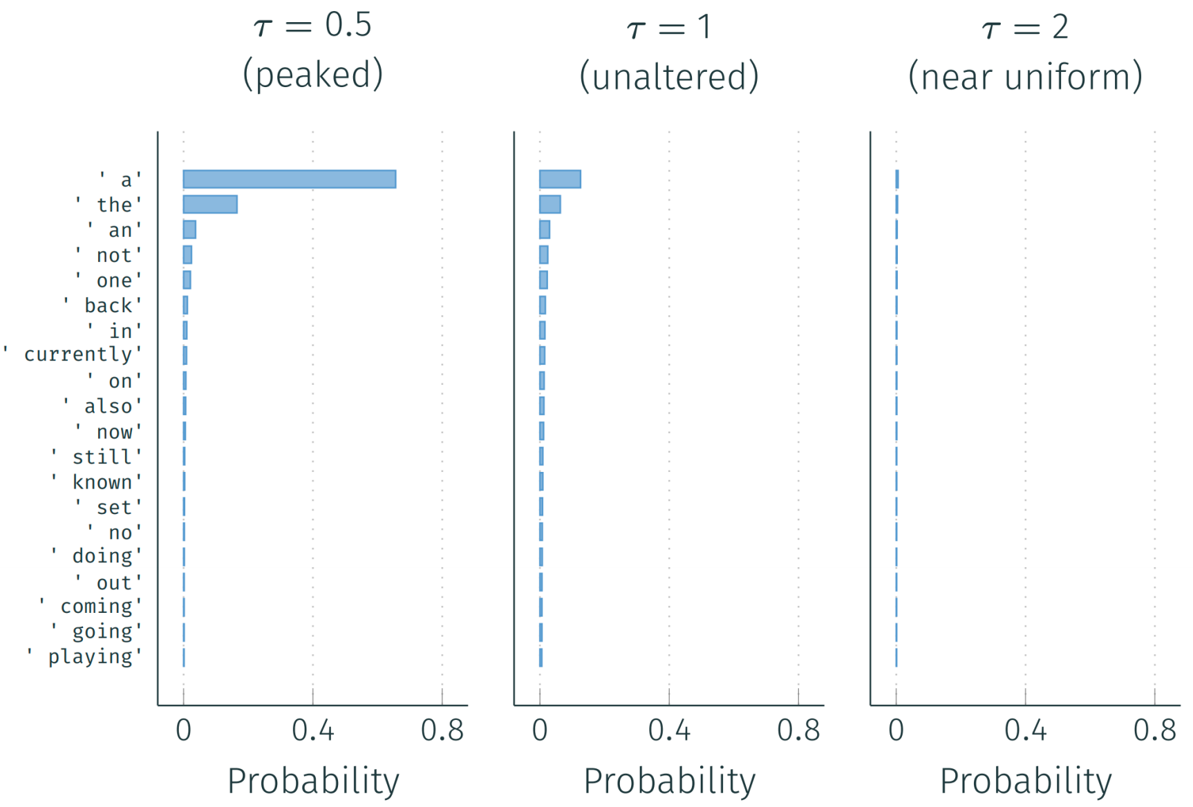
Temperature Sampling: Make distribution more peaked \[ \text{softmax}(x, \tau) = \frac{\exp(x/\tau)}{\sum_i \exp(x_i/\tau)} \]

Temperature	Parameter	Pro	Con
High	\(\tau \geq 1\)	Diverse	Incoherent
Low	\(\tau < 1\)	Coherent	Repetitive

HuggingFace interface:

# Top-k
model.generate(do_sample=True, top_k=20)

# Top-p
model.generate(do_sample=True, top_p=0.9)

# Temperature
model.generate(do_sample=True, temperature=0.7)

Other Truncation Strategies

Method	Threshold Strategy
Top-\(k\)	Sample from \(k\)-most-probable
Top-\(p\)	Cumulative probability at most \(p\)
\(\epsilon\)	Probability at least \(\epsilon\)
\(\eta\)	Min prob. proportional to entropy
Min-\(p\)	Prob. at least \(p_{\min}\) scaled by max token prob.

Speeding Up Decoding

Why is Decoding Slow?

Time bottleneck: \[ \text{time} = \max\left(\frac{\text{OperationFLOPs}}{\text{DeviceFLOP/s}}, \frac{\text{DataTransferred(GB)}}{\text{MemoryBandwidth(GB/s)}}\right) \]

Compute-bound: e.g., \(A = BC\) (matrix multiplication)
Memory-bound: e.g., \(a = Bx\) (matrix-vector multiplication)
Decoding one token is typically memory-bound

Metrics

Latency: How long does a user wait? - Time to first token, time per request

Throughput: How many requests completed per second? - Tokens per second, requests per second

Key-Value Cache

Problem: Without caching, computing attention requires \(O(T^2)\) recomputation.

Solution: Store previously computed keys and values.

At step \(t\) of decoding (1 layer, 1 head): \[ \begin{align} q_t &= h_t W_q \in \mathbb{R}^{1 \times d_k} \\ k_t &= h_t W_K \in \mathbb{R}^{1 \times d_k} \\ v_t &= h_t W_V \in \mathbb{R}^{1 \times d_v} \end{align} \]

Cached: \(K_{1:t-1} \in \mathbb{R}^{(t-1) \times d_k}\), \(V_{1:t-1} \in \mathbb{R}^{(t-1) \times d_v}\)

Append \(k_t\) to \(K_{1:t-1}\) and \(v_t\) to \(V_{1:t-1}\): \[ z_t = \text{softmax}\left(\frac{q_t K_{1:t}^T}{\sqrt{d_k}}\right) V_{1:t} \]

Speedup: Reduces \(O(T^2)\) to \(O(T)\) computation.

Speeding Up a Single Token

Goal	Strategy	Examples
Reduce memory bandwidth	Quantization, distillation, architecture	GPTQ, AWQ, GQA/MQA
Increase FLOP/s	Optimize operations on hardware	FlashAttention, torch.compile
Decrease FLOPs	Reduce FLOPs in architecture	Mixture-of-Experts, Mamba

Speeding Up a Full Sequence

Strategy	Idea	Examples
Parallelize over time	Draft tokens cheaply, verify in parallel	Speculative decoding
Parallelize over time	Generate multiple tokens in parallel	Non-autoregressive models

Speculative Decoding: 1. Use small draft model \(q\) to generate tokens ahead 2. Large model \(p\) processes drafted tokens in parallel 3. Accept with probability: \(\alpha_i = \min\left(1, \frac{p(\text{token} | \ldots)}{q(\text{token} | \ldots)}\right)\)

Speeding Up Multiple Sequences

Strategy	Idea	Examples
State re-use	Shared prefixes \(\Rightarrow\) shared KV cache	PagedAttention, RadixAttention
Improved batching	Better scheduling	Continuous batching
Program-level optimization	Optimize full generation graph	SGLang, DSPy

Summary

Decoding as optimization: Greedy, beam search, MAP (A fixed route the maxmize the probability )
- Pitfalls: degeneracy, atypicality, probability spread
Sampling: Ancestral, top-k, top-p, temperature. (change the probability distribution for the following sampling)
- Addresses tail probability and diversity issues
Efficient inference: KV cache, speculative decoding, batching
- Critical for deployment at scale

A key takeaway is that the Beam search or Greedy is search-based, it wants to get a fiexd optimized output, but Samlping introduces diversity or variance to generate more creative answers and may get different answers.