15618 Assignment 1 Report
15618 Assignment 1 Exploring Multi-Core and SIMD Parallelism Report
Problem 1: Parallel Fractal Generation Using Pthreads
1.1 Speedup Graph
Implementation: Multi-threaded Mandelbrot generation using horizontal striping (spatial decomposition). Each thread processes consecutive rows. For cases where the number of rows (900) is not evenly divisible by the number of threads, the first (900 % T) threads are assigned one additional row to ensure all rows are processed.

Note: 16 threads use the same 8 physical cores via hyperthreading.
And speedup is not linear. With 8 cores, we achieve only 3.97× speedup (49.6% efficiency) instead of the ideal 8×.
Hypothesis: Load Imbalance:
The horizontal striping strategy creates severe load imbalance because:
- Top/bottom rows: Points far from Mandelbrot boundary diverge quickly (~10-50 iterations)
- Middle rows: Points near the boundary require maximum iterations (256)
- Result: Threads assigned to middle rows work significantly longer
Since total time equals the slowest thread, unbalanced work significantly reduces speedup.
Key Obeservation:
The sharp drop in efficiency from 2 threads (98%) to 4 threads (60%) confirms that load imbalance is the dominant performance bottleneck, not hardware limitations.
1.2 Per-Thread Timing Measurements
To verify the load imbalance hypothesis from Section 1.1, I instrumented the code by adding timing measurements at the beginning and end of workerThreadStart() using CycleTimer::currentSeconds().
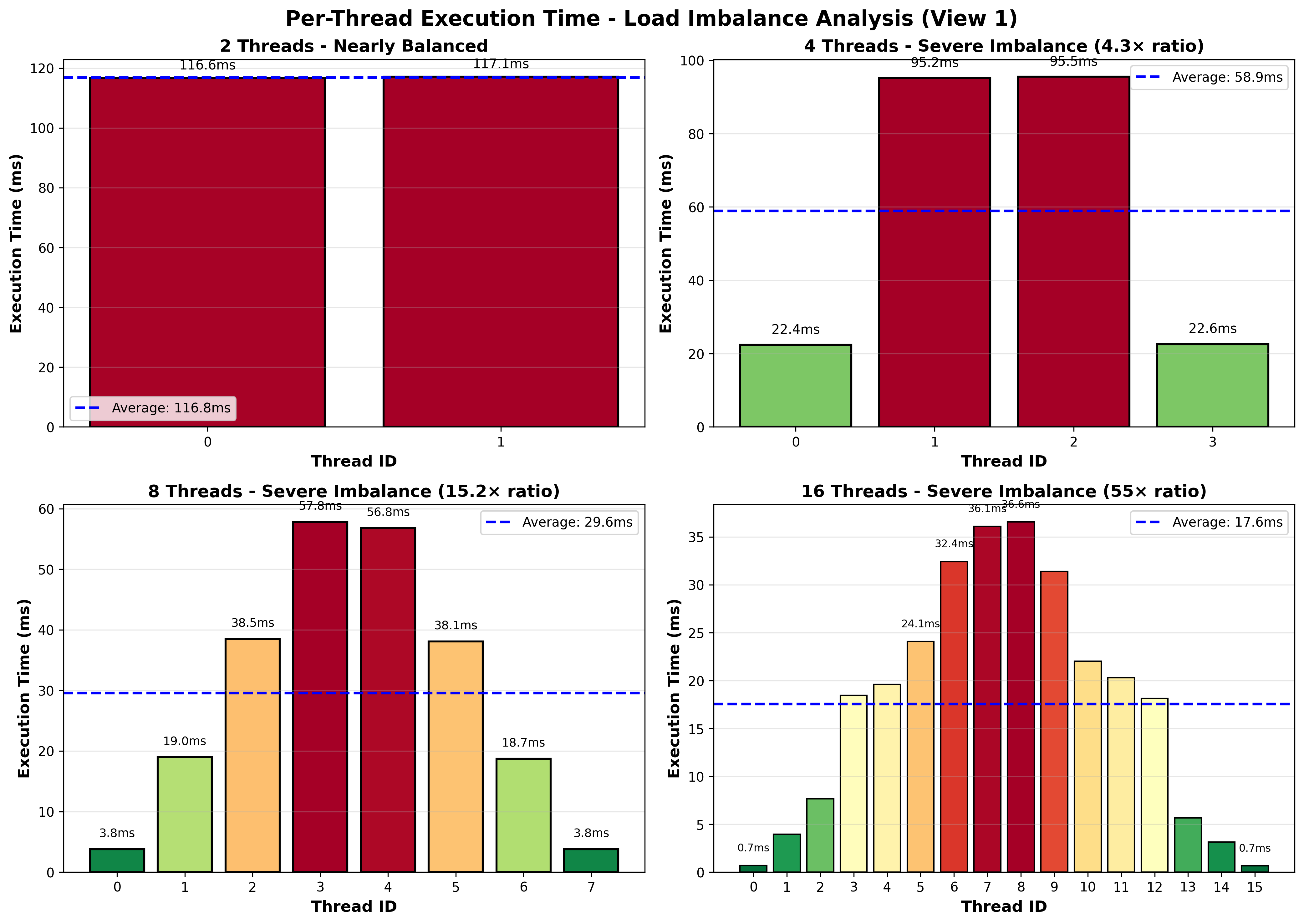
Analysis: Load Imbalance Confirmed
The timing visualization clearly shows severe load imbalance across all configurations. The color gradient reveals the problem: threads processing top and bottom rows (green bars) finish quickly, while threads handling middle rows (red bars) take significantly longer. This pattern directly corresponds to the Mandelbrot set’s computational structure—boundary regions require maximum iterations while outer regions diverge quickly.
For 4 threads, this imbalance means two threads sit idle for most of the execution time while two others continue working, wasting half the available CPU capacity. With 8 threads, the problem worsens: most threads finish early and wait for the few threads stuck processing expensive boundary rows. This uneven distribution explains why we achieve only 3.97× speedup with 8 cores instead of the ideal 8×—the execution time is bottlenecked by the slowest thread, not the average workload.
1.3 Improve Speedup
Strategy: Interleaved Row Assignment
Instead of horizontal striping (consecutive rows per thread), I implemented interleaved assignment where thread i processes rows i, i+T, i+2T, i+3T, …, where T is the total number of threads.
This simple static assignment ensures each thread processes a mix of computationally cheap rows (top/bottom of image) and expensive rows (near Mandelbrot boundary), automatically balancing the workload without any synchronization.
| Threads | View 1 Speedup | View 2 Speedup |
|---|---|---|
| 4 | 3.84× | 3.82× |
| 8 | 7.56× | 7.53× |
| 16 | 7.61× | 7.35× |
Scaling Behavior Analysis:
4→8 threads (4→8 cores): Speedup nearly doubles, demonstrating excellent scaling as each additional thread runs on a dedicated physical core with full computational resources.
8→16 threads (8 cores with hyperthreading): Performance improvement is limited or even decreases (View 2). Since both configurations share the same 8 physical cores, the 16 threads compete for execution units and cache via hyperthreading. For compute-intensive Mandelbrot workloads with minimal memory stalls, hyperthreading provides little benefit.
Problem 2: Vectorizing Code Using SIMD Intrinsics
2.1 clampedExpVector
The implementation follows the exponentiation by squaring algorithm and processes W elements in parallel per vector instruction.
Key Implementation Details:
- Loop Structure: Process array in chunks of VECTOR_WIDTH, with each iteration handling one vector of elements
- Mask Management: Use maskActive to track which lanes still have exponent > 0, terminating the loop when all lanes complete
- Boundary Handling: Dynamically create masks using _cmu418_init_ones(count) to correctly handle cases where N is not a multiple of W
- Result Clamping: Vectorized the clamping logic to limit results exceeding 4.18
Correctness: Passed all test cases including non-aligned array sizes (e.g., N=3, N=10, N=100)
2.2 Vector Width Sweep Experiments
Experimental Setup: Ran ./vrun -s 10000 with VECTOR_WIDTH ∈ {2, 4, 8, 16, 32}
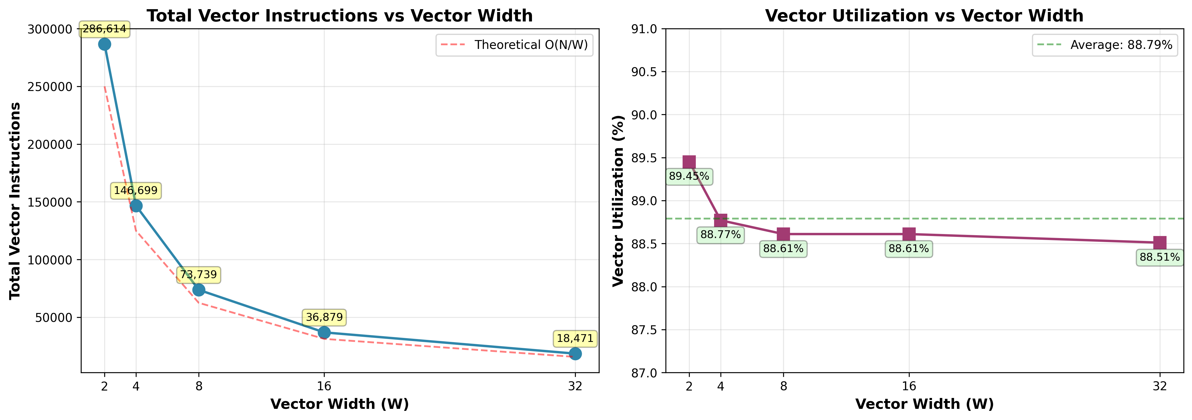
Vector Utilization Analysis
Observation: Vector utilization remains high (88.51%-89.45%) across all vector widths, with only 0.94% degradation as W increases from 2 to 32. This demonstrates low sensitivity to vector width.
This is because the iteration counts are proportional to log₂(exponent), meaning a 10× difference in exponents (e.g., 100 vs 1000) results in only ~3 additional iterations. Since vector instructions must wait for the slowest lane to complete, each vector’s iteration count is determined by the element with the maximum iterations. This low variance ensures elements within a vector finish at similar times, minimizing idle lanes regardless of vector width.
Number of Vector Instructions Analysis
Observation: Total vector instructions decrease from 286,614 (W=2) to 18,471 (W=32), approximately halving with each doubling of vector width. The measured instruction counts closely follow the theoretical O(N/W) curve (red dashed line), confirming near-ideal scaling.
The total instruction count is determined by how many times the outer loop runs. When vector width doubles (e.g., W=4 to W=8), each vector instruction can process twice as many elements, so the outer loop only needs to run half as many times. Since the work inside each loop iteration stays the same, doubling W directly halves the total instructions. This 93.6% reduction from W=2 to W=32 demonstrates that vectorization delivers the expected linear speedup.
2.3 arraySumVector
Implemented a tree reduction algorithm achieving O(N/W + log₂W) span complexity:
Algorithm:
- Phase 1 - Vector Accumulation (O(N/W)): Sum all array elements into a single vector register using vector addition
- Phase 2 - Tree Reduction (O(log₂W)): Reduce W elements within the vector to a single scalar using hadd and interleave operations in log₂W rounds
Correctness: Passed all tests for W = 2, 4, 8, 16
Problem 3: Parallel Fractal Generation Using ISPC
3.1 Part 1: ISPC SIMD Parallelization Analysis

8x theoretical maximum speedup
The ISPC compiler is configured to emit 8-way AVX2 SIMD instructions, which can process 8 floating-point values simultaneously. Therefore, the theoretical maximum speedup is 8x compared to the serial implementation.
SIMD Divergence (Stall)
The observed average speedup of 4.48x is only 56% of the theoretical 8x maximum because different pixels require different numbers of iterations to determine if they’re in the Mandelbrot set—when processing 8 pixels together in SIMD, some finish quickly while others take much longer, forcing all lanes to wait for the slowest one, which wastes computation on idle lanes.
Performance Variation Across Views
Different views show speedups ranging from 4.01x to 4.88x (View 6: 4.88x best, View 5: 4.01x worst). Views with complex fractal boundaries have neighboring pixels with very different iteration counts, causing more SIMD lanes to wait idle, while views with smoother regions have pixels that finish at similar times, reducing wasted computation.
3.2 Part 2: ISPC Tasks
Speedup with –tasks
| Implementation | Time (ms) | Speedup vs Serial | Speedup vs ISPC |
|---|---|---|---|
| Serial | 176.369 | 1.00x | - |
| ISPC (SIMD only) | 37.019 | 4.76x | 1.00x |
| ISPC + Tasks (2 tasks) | 18.721 | 9.42x | 1.98x |
The 2x improvement from tasks makes sense because the current implementation only creates 2 tasks, utilizing only 2 out of 8 cores. Performance can be significantly improved by increasing the task count.
Find the optimal tasks count
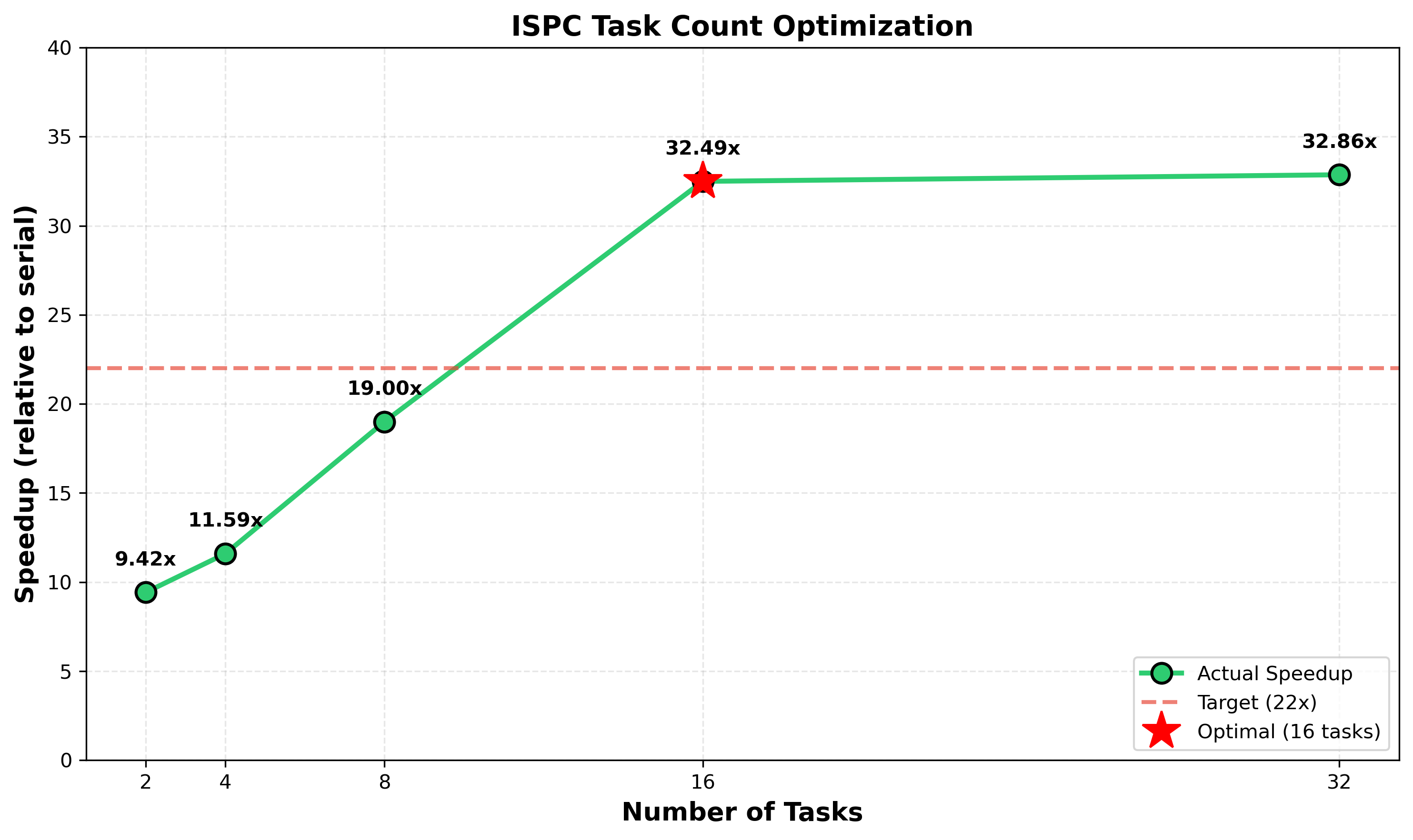
Optimal number of tasks is 16
The system has 8 physical cores with hyper-threading, allowing 16 hardware threads to run simultaneously. Using 16 tasks achieves the best performance (32.49× speedup) because:
- Matches hardware capacity: 16 tasks fully utilize all 16 hardware threads, keeping all execution units busy.
- Better load balancing: The Mandelbrot computation has uneven workload—fractal boundaries require many more iterations than solid regions. With only 2 tasks, one task might get stuck on a heavy region while the other finishes early. With 16 smaller tasks, work distributes more evenly across cores.
- Diminishing returns beyond 16: Using 32 tasks (32.86×) shows minimal improvement over 16 tasks because task scheduling overhead increases while load balancing benefits plateau.
Pthread vs ISPC Tasks
Pthreads are OS-level threads with significant overhead. Launching 10,000 of them would likely crash or severely slow down a system due to excessive memory consumption and context switching.
In contrast, ISPC tasks are lightweight logical units. The runtime maps them onto a small, fixed thread pool (typically matching the CPU core count). Launching 10,000 tasks is efficient because they are scheduled via a task queue.
The key difference is Pthreads are for coarse-grained parallelism (fewer tasks, high overhead), while ISPC tasks enable fine-grained data parallelism (many tasks, low overhead). This makes ISPC ideal for SPMD-style operations like pixel-level processing.
Problem 4: Iterative Square Root
4.1 Speedup
1 | Serial: 682.707 ms |
4.2 initGood
Implementation: Set all values to
2.999f
1 | Serial: 1698.132 ms |
This choice maximizes speedup by:
Perfect SIMD efficiency: All elements converge in identical iterations, eliminating lane divergence. Every SIMD lane performs the same amount of work and finishes simultaneously with no idle waiting. SIMD speedup improved from 4.69x (random) to 5.71x.
Maximum multi-core benefit with hyper-threading: The uniform heavy workload enables exceptional multi-core scaling. Multi-core speedup reached 8.76x, exceeding the baseline 7.25x. This demonstrates the hyper-threading effect mentioned in the assignment - when all threads execute identical heavy workloads, hyper-threading can provide additional performance beyond the physical core count.
4.3 initBad
Implementation: Alternate between
2.999f and 1.0f every 8 elements
1 | Serial: 234.384 ms |
Choice of values: 2.999f requires much
more iterations, while 1.0f requires ~0 iterations
(matching the initial guess). This creates maximum iteration count
divergence within each SIMD gang.
SIMD performance: This pattern creates maximum work divergence within each SIMD vector (gang size = 8), with 1 slow element and 7 fast elements per vector. SIMD operates in lockstep where all lanes must wait for the slowest lane, performance drops below serial execution (0.79x).
Multi-core performance: Multi-core speedup remains very high at 8.77x, nearly identical to initGood (8.76x). The pattern repeats uniformly across the array (every 8th element is slow), ensuring balanced workload distribution across threads despite severe SIMD inefficiency within individual vectors.
Problem 5: BLAS saxpy
5.1 Analysis of saxpy’s performance
| Version | Time (ms) | Bandwidth (GB/s) | Performance (GFLOPS) | Speedup |
|---|---|---|---|---|
| Serial | 11.356 | 26.243 | 1.761 | 1.00x |
| Streaming | 11.242 | 26.509 | 1.779 | 1.01x |
| ISPC | 11.315 | 26.339 | 1.768 | 1.00x |
| Task ISPC | 11.133 | 26.768 | 1.796 | 1.02x |
The workload is memory bandwidth-bound. Saxpy accesses large amounts of data but performs only 2 FLOPs. The processor spends far more time waiting for memory than computing. Despite saxpy being trivially parallelizable, ISPC and multi-core execution provide minimal ~1.00x speedup. All implementations saturate at approximately 26-27 GB/s, indicating we’ve reached the memory bandwidth limit.
The program cannot be substantially improved through parallelism alone. Adding more cores or SIMD lanes doesn’t help when serial execution already maximize the memory bandwidth. Potential improvements require reducing memory traffic (e.g., using non-temporal stores for the result vector to avoid cache pollution, reducing bandwidth from 4N to 3N floats) or upgrading to higher bandwidth memory hardware.
5.2 Extra Credit: Why 4N instead of 3N?
I think it’s because the cache’s behavior. Modern CPUs use a write-allocate cache policy, meaning write operations must firstly load the target data into the cache before modifying it. This is required for cache coherence and locality optimization. So the additional N floats is reading result cache lines.
5.3 Extra Credit: What else factors could affect?
The observed bandwidth of 26-27 GB/s represents typical efficiency for DDR4 memory systems. The gap between observed and theoretical peak is due to:
- DRAM timing overhead: DDR4 requires mandatory delays between operations (CAS latency, row precharge time, refresh cycles) during which the memory bus is idle. These timing constraints typically reduce effective bandwidth to 60-70% of theoretical peak.
- Memory controller efficiency: Bank conflicts, channel arbitration, and command scheduling in the memory controller add additional overhead.
5.4 Extra Credit: Non-temporal Store Optimization
Implementation: Modified saxpyStreaming() using SSE
intrinsics with _mm_stream_ps to bypass cache.
| Version | Time (ms) | Bandwidth (GB/s) | Performance (GFLOPS) | Speedup |
|---|---|---|---|---|
| Serial | 11.124 | 26.791 | 1.798 | 1.00x |
| Streaming | 8.138 | 36.623 | 2.458 | 1.37x |
| ISPC | 11.201 | 26.608 | 1.786 | 0.99x |
| Task ISPC | 11.125 | 26.789 | 1.798 | 1.00x |
Non-temporal stores reduce memory traffic from 4N to 3N floats, achieving 1.37x speedup and bandwidth improvement from 26.8 GB/s to 36.6 GB/s.