CS336-Lec4 Mixture of Experts

In the modern competition of ultra-large-scale LLMs, the Mixture of Experts (MoE) model has become a core technology for achieving “trillions of parameters” and “controllable computational costs.”

Core Definition of MoE

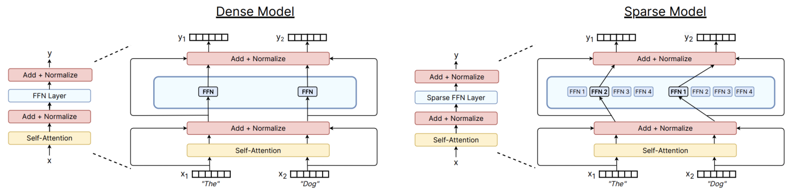
Traditional Transformer models are dense, where every Token activates all parameters. The basic idea of MoE is to replace the massive FFN with multiple parallel expert networks, and then add a routing layer to determine which expert(s) a Token will enter.

The output \(\mathbf{h}_t^l\) of the MoE layer at position \(t\) can be represented as the weighted sum of the outputs from the selected experts: \[ \mathbf{h}_t^l = \sum_{i=1}^{N} \left( g_{i,t} \cdot \text{FFN}_i (\mathbf{u}_t^l) \right) + \mathbf{u}_t^l \] where:

\(N\) is the total number of experts.
\(\mathbf{u}_t^l\) is the input Token vector for that layer.
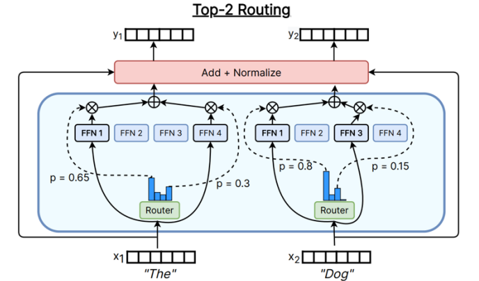
\(g_{i,t}\) is the Gating Weight computed by the router, typically calculated via Top-K routing, as discussed in the next section.

Routing Mechanism

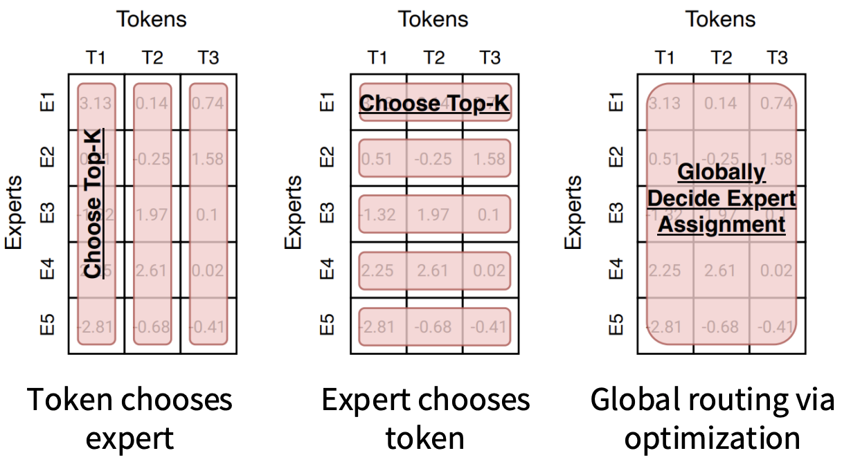
The routing function is a very important part of MoE, as it determines the efficiency of parameter utilization. We will first introduce some possible implementations of routing mechanisms, which can generally be categorized into those that require Learning and those that do not:

Learning-required mechanisms include Top-K and RL-based routing.
Non-learning mechanisms include Hash and Base Routing.

Here, we will briefly introduce the two non-learning mechanisms:

Hash Routing: Uses a fixed hash function to assign Tokens to experts. Since the routing is fixed, there is no need to learn the Router parameters, thus avoiding non-differentiability issues.
BASE Routing: Transforms the routing decision into a Linear Assignment problem to find the optimal global matching.

However, most models currently use Choose Top-K, which also has several variants.

Mathematical Details of Top-K Routing (Mainstream Approach)

The router first calculates the relevance score \(s_{i,t}\) between the Token and the expert embedding vector \(e_i\): \[ s_{i,t} = \text{Softmax}_i (\mathbf{u}_t^{lT} e_i^l) \] Then, it implements sparse activation through the Top-K operator: \[ g_{i,t} = \begin{cases} s_{i,t}, & s_{i,t} \in \text{TopK}(\{s_{j,t} | 1 \le j \le N\}, K) \\ 0, & \text{otherwise} \end{cases} \]

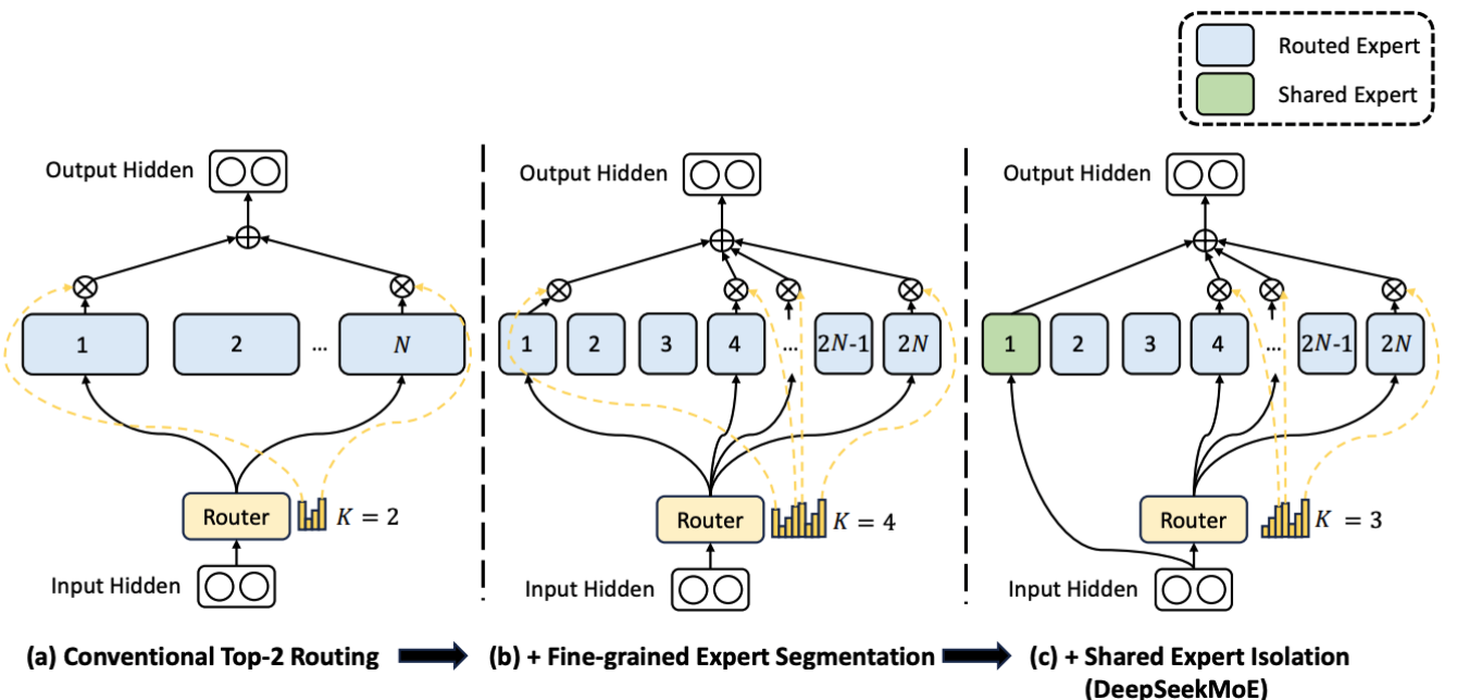
Modern Architecture Variant: DeepSeekMoE

DeepSeek introduces more refined designs to enhance the effectiveness of MoE:

Fine-grained expert segmentation: Splits large experts into multiple smaller experts (e.g., \(2N\)), allowing for more precise knowledge combinations.
Shared Expert Isolation: Sets fixed experts that handle all Tokens sharing basic common knowledge, reducing redundancy among routing experts.

Stability of Training

The core challenge of MoE lies in how to train it stably. To improve training efficiency, the model needs to exhibit sparsity, but the sparse gating mechanism (Top-K) is Non-differentiable. Additionally, we need to maintain load balancing among experts; without constraints on the Router, traffic can concentrate on certain experts, leading to others not being trained and becoming “dead experts.” We have the following solutions to address this issue.

Reinforcement Learning

The principle is straightforward: treat the entire Router as an agent and the Tokens as actions, using reinforcement learning algorithms to optimize the routing strategy based on the final loss (as a reward).

However, this method is not commonly used; while logically correct, it suffers from high gradient variance and computational complexity, making it less favorable in large-scale training compared to other solutions.

Stochastic Perturbations

The principle is to add Gaussian noise or Jitter to the routing logits, forcing the model to explore some unconventional paths. \[ H(x)_i = (x \cdot W_g)_i + \text{StandardNormal}() \cdot \text{Softplus}((x \cdot W_{noise})_i) \] Even if the initial weights are poor, randomness allows each expert to have a chance to be trained, making the routing more robust and avoiding the emergence of dead experts.

Auxiliary Loss

To ensure that each expert shares the task evenly, an auxiliary loss is introduced, meaning that experts used more frequently receive greater penalties, with the minimum loss ensuring that tasks are evenly distributed among experts: \[ \text{Loss}_{aux} = \alpha \cdot N \cdot \sum_{i=1}^N f_i \cdot P_i \] where:

\(f_i\) (distribution ratio): Represents the proportion of Tokens assigned to expert \(i\) in that batch.

\[ f_{i} = \frac{1}{T} \sum_{x \in \mathcal{B}} \mathbb{I}\{argmax \ p(x) = i\} \]

\(P_i\) (routing probability ratio): Represents the total probability assigned to expert \(i\) by the Router.

\[ P_{i} = \frac{1}{T} \sum_{x \in \mathcal{B}} p_{i}(x) \]

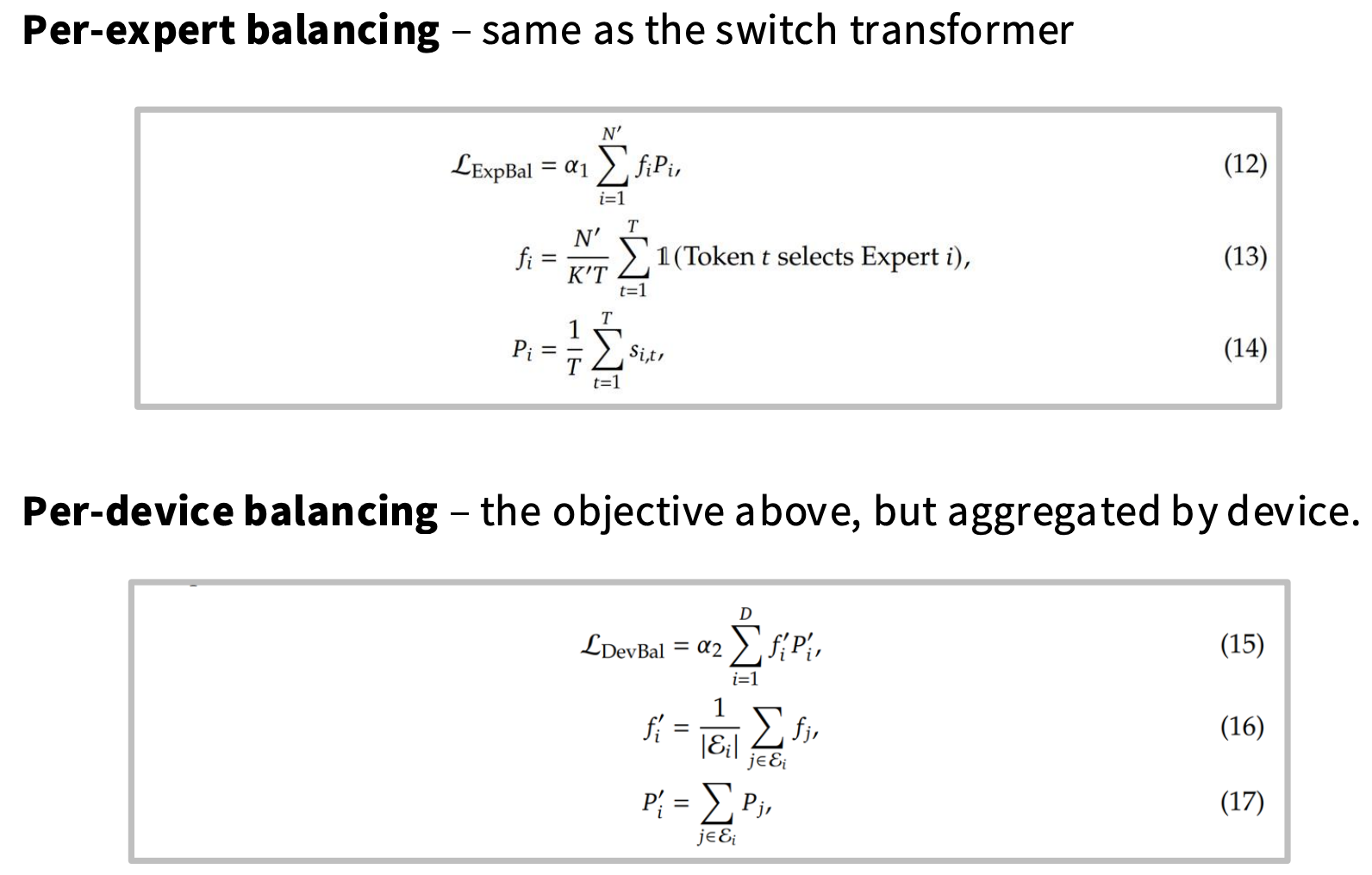
Implementation of DeepSeek Variants

DeepSeek v1-2 (Dual Balance of Experts and Devices): Introduces Per-expert Loss (consistent with Switch Transformer) to ensure balance among experts, and Per-device Loss to ensure balance in cross-GPU communication (All-to-All).

DeepSeek v3 (No Auxiliary Loss Balance): Introduces the Per-expert Bias (\(b_i\)) mechanism: \[ S_{i,t}^{\prime} = \begin{cases} s_{i,t}, & s_{i,t}+b_{i} \in Topk(\{s_{j,t}+b_{j} | 1 \le j \le N_{r}\}, K_{r}) \\ 0, & \text{otherwise} \end{cases} \] Adjusts the bias \(b_i\) through online learning to achieve balance without disrupting the gradient of the main loss (Auxiliary-loss-free).

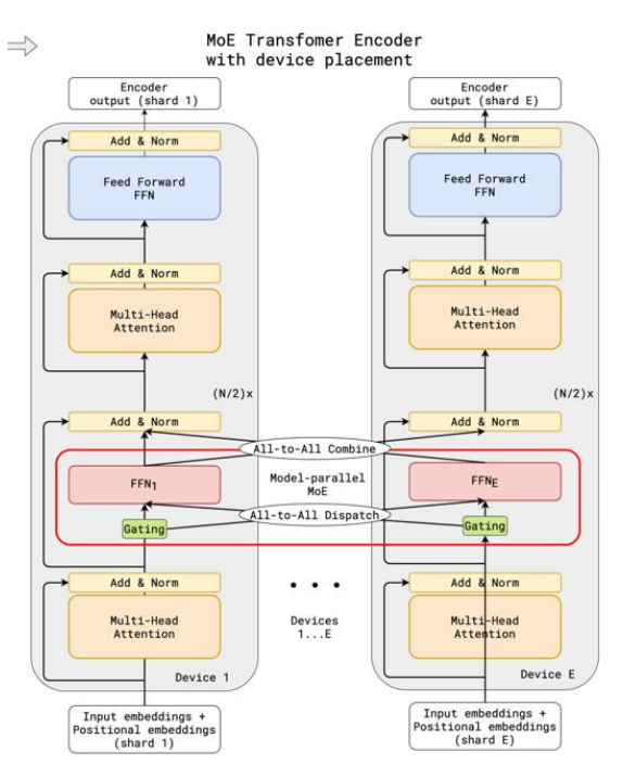
System Optimization: Distributed Parallelism and Computational Optimization

Due to the enormous parameter scale, the physical implementation of MoE heavily relies on parallelization.

1. Device Placement

All-to-All Dispatch: Tokens are distributed across devices to the corresponding expert nodes based on routing results.
All-to-All Combine: Computation results are returned while maintaining sequence order.

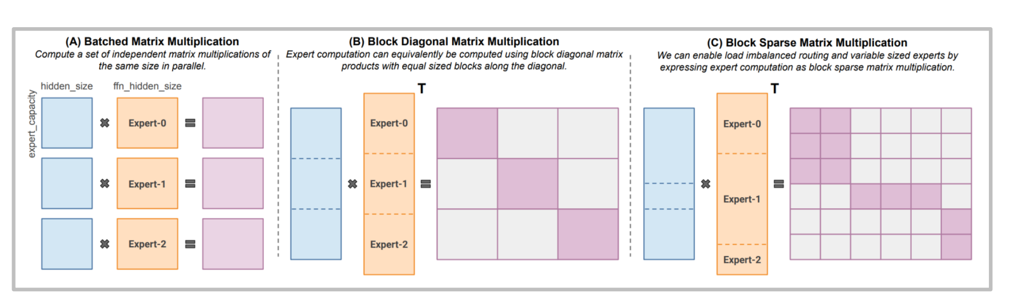
2. Computational Operator Optimization (MegaBlocks)

Traditional matrix multiplication is inefficient when facing uneven loads. Libraries like MegaBlocks introduce Block Sparse MM, which can efficiently handle variable-length expert computations, avoiding resource waste due to padding.

Advanced Techniques

z-loss (Numerical Smoothing): To prevent Softmax from overflowing at low precision, it penalizes \(\log^2 Z\) (where \(Z\) is the partition function) to force logits to remain within a safe range.

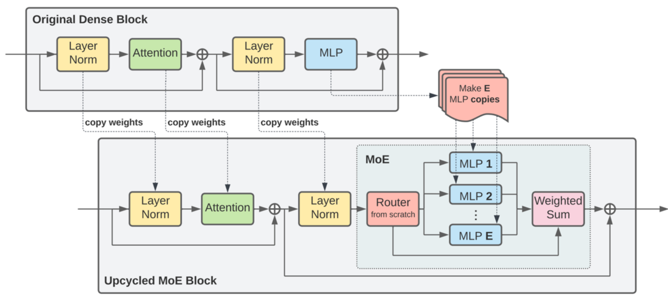
Upcycling: Trained dense model FFN weights can be cloned multiple times as initial values for MoE experts, significantly shortening the training time from scratch, showing substantial improvements on some models.

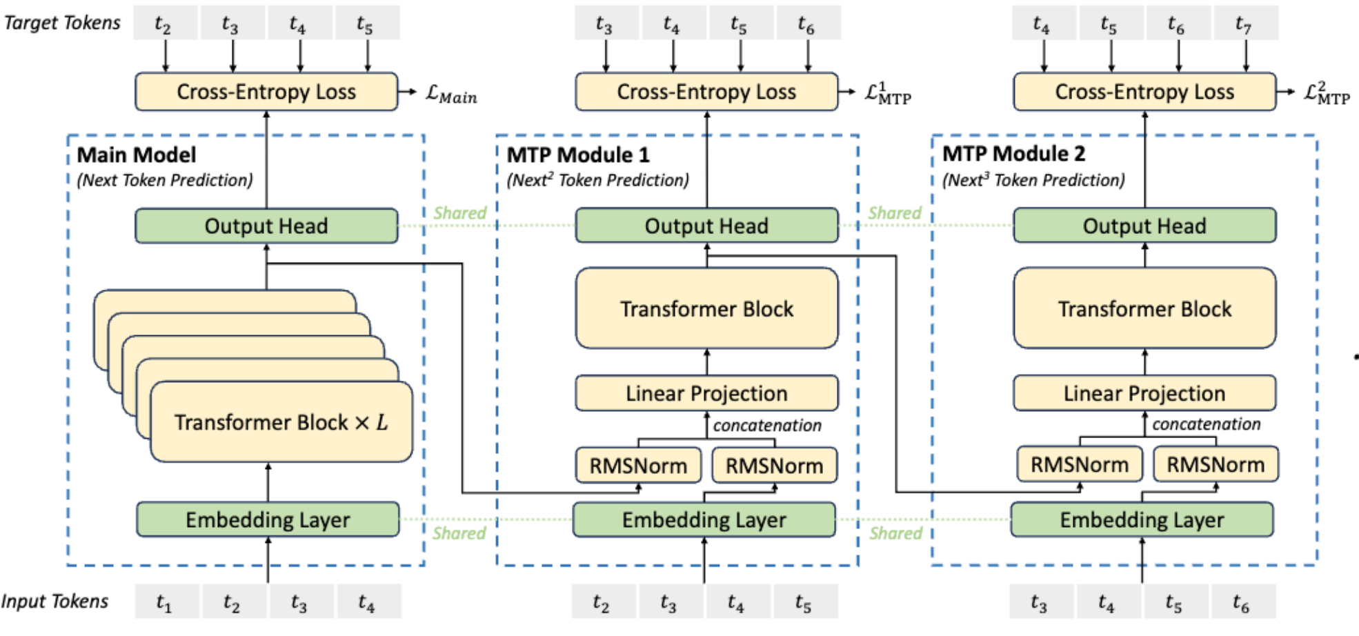
MTP (Multi-Token Prediction): A technique used in DeepSeek v3. It adds a lightweight module outside the main model to predict multiple future Tokens at once, enhancing the model’s ability to model long texts.

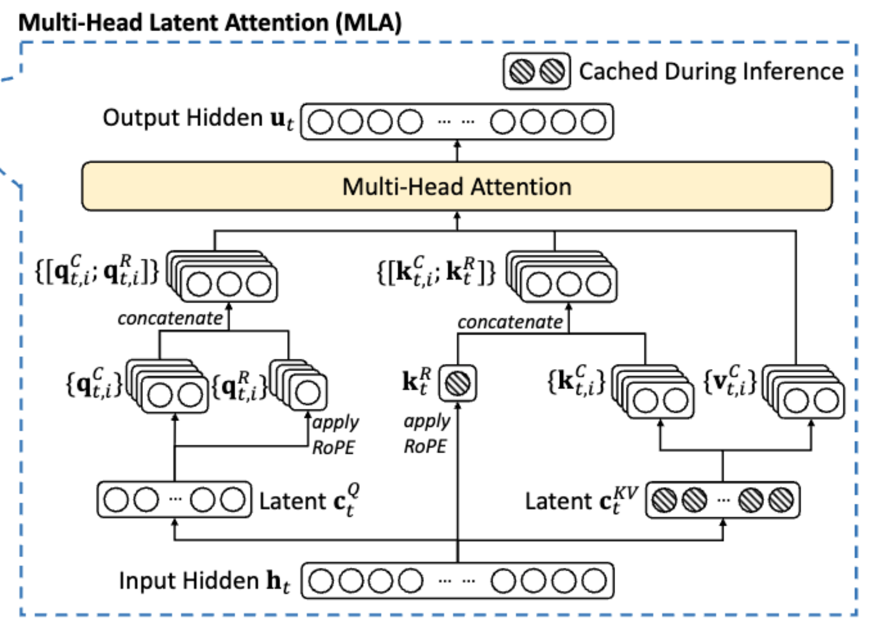
MLA (Multi-Head Latent Attention): A key solution in DeepSeek v3 to the KV Cache bottleneck. It compresses Q, K, and V into a low-dimensional “latent” space, requiring only a small latent vector \(c_t^{KV}\) to be cached during inference, significantly reducing memory usage. Additionally, through a decoupled design, some dimensions do not participate in compression (a hard rule set during model architecture) to accommodate rotary position encoding (RoPE), resolving conflicts between position encoding and compressed cache.

Why is caching avoided? A: The reconstruction matrix \(W^{UK}\) can be directly absorbed into the projection of the query matrix Q. This means that during inference, we only need to cache the low-dimensional \(c_t^{KV}\)** in memory, rather than caching the reconstructed multi-head K and V.

\[ \text{Score} = (h W_Q)^T \times (W_{UK} c_t^{KV}) = h \cdot (W_Q W_{UK}) \cdot c_t^{KV} \]

Why should RoPE be decoupled? Can’t we just add RoPE directly in the latent space? A: No, looking directly at the formula, we cannot merge the matrices into one, which would require us to restore the Key, thus ruining the plan to save memory.

\[ \text{Score} = (R_m h W_Q)^T \times (R_n W_{UK} c_n^{KV}) = h W_Q \cdot (R_m^T R_n) \cdot W_{UK} c_n^{KV} \]