CS336-Lec3 Architectures & Hyperparameters

Overview of Original vs. Modern Transformer

Feature	Original Transformer	Modern Variants	Optimization Goals/Advantages
Layer Normalization	Post-Norm: After each sub-layer (Attention/FFN).	Pre-Norm: Before each sub-layer.	Improves training stability of deep models and accelerates convergence.
Normalization Type	LayerNorm: Normalizes mean and variance	RMSNorm: Normalizes only variance, does not subtract mean, no bias term.	Faster computation, fewer parameters, no significant drop in performance.
Bias Term	FFN and linear layers have bias term \(\boldsymbol{b}\).	Linear layers (including normalization layers) do not have bias term.	Reduces memory usage and improves optimization stability.
Positional Encoding	Sine/Cosine Encoding: Adds positional information to embeddings.	Rotary Positional Encoding (RoPE): Encodes positional information into the rotation operation of query and key (Q/K) vectors.	Better captures relative positional information, has become standard for most SOTA models (like LLaMA) after 2024.
FFN Activation Function	ReLU	SwiGLU/GeGLU: A gated activation function.	Generally outperforms ReLU and GeLU, with more consistent gains.
Layer Connection	Serial: Computes Attention first, then computes MLP.	Serial or Parallel: Attention and MLP compute in parallel.	Parallel structure can achieve about 15% training speedup through matrix multiplication fusion during large-scale training.

Normalization

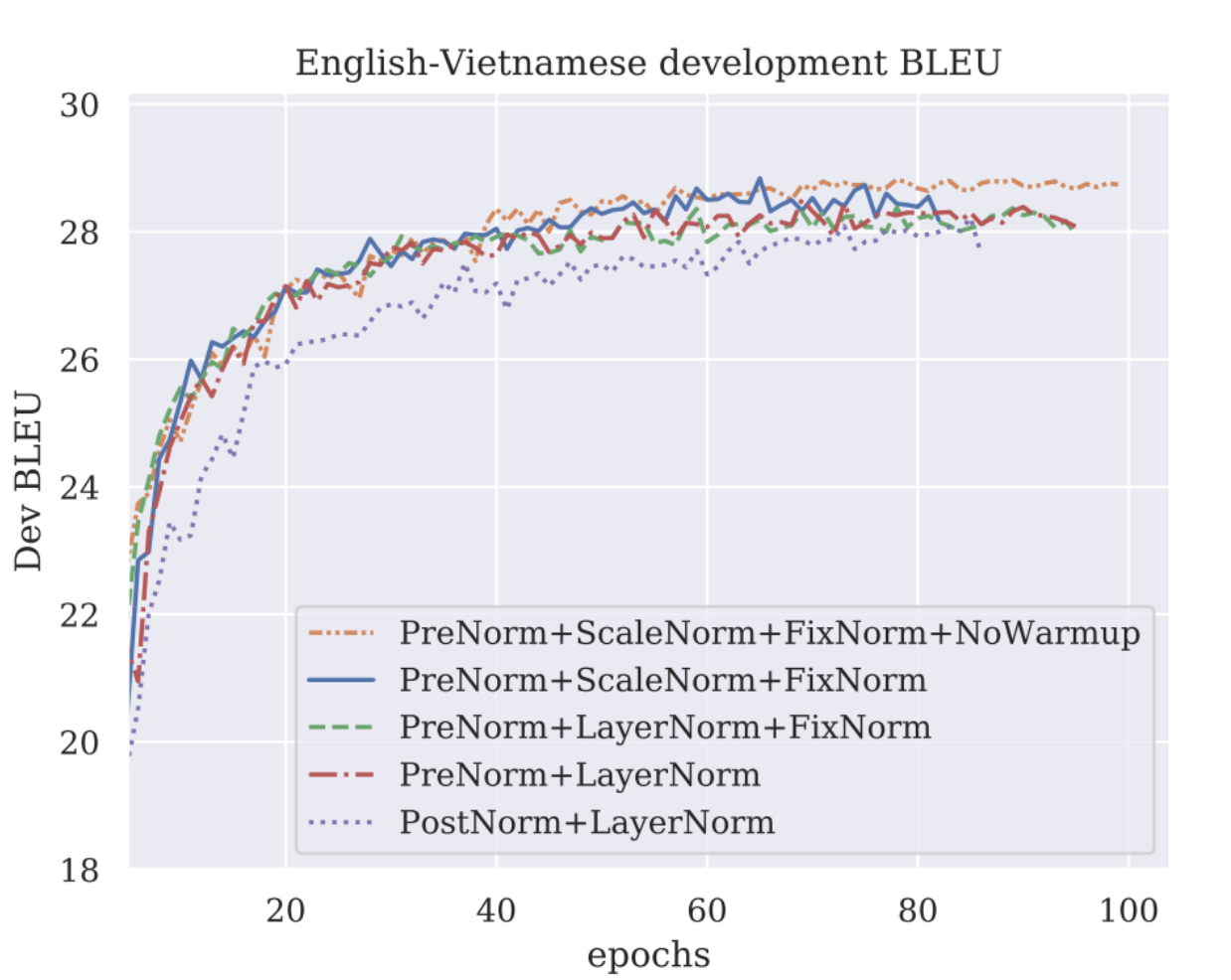
In the Transformer architecture, the position of normalization layers is crucial for the stability and efficiency of model training. Modern LLMs have almost uniformly discarded the original normalization positions in favor of more stable strategies.

Pre-Norm vs. Post-Norm

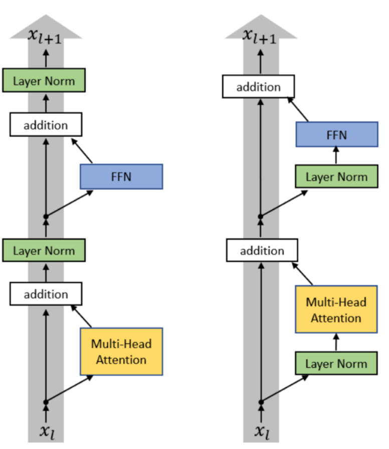
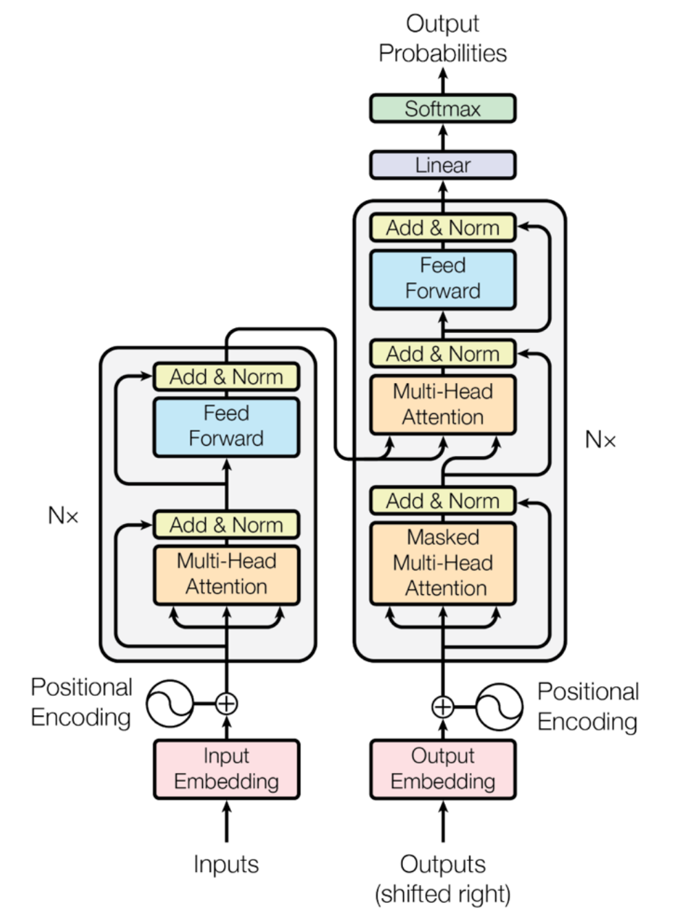
• Post-Norm (Original Transformer): Normalization occurs after the residual connection of each sub-layer (like Multi-Head Attention or FFN). This structure can lead to gradient vanishing or gradient explosion when training deep models, affecting training stability.
• Pre-Norm (Modern LLM): Normalization occurs before each sub-layer. This placement ensures that the main path signal of the residual connection maintains a good scale, greatly improving gradient propagation and enhancing training stability in deep networks.

It is worth noting that almost all modern LMs use pre-norm (but BERT was post-norm).

LayerNorm vs. RMSNorm

The original Transformer uses LayerNorm, while modern LLMs tend to prefer RMSNorm. There are core differences in mathematical and engineering efficiency between these two methods.

LayerNorm: \[ y=\frac{\boldsymbol{x}-E[\boldsymbol{x}]}{\sqrt{\text{Var}[\boldsymbol{x}]+\epsilon}} \cdot \gamma+\beta \]

• The above is to center and normalize the input \(\boldsymbol{x}\) (e.g., a \(d_{model}\) dimensional feature vector of a token) of a layer in the neural network, making its mean 0 and variance 1.
• \(\gamma\) and \(\beta\) are the scaling parameter and offset parameter, respectively, which are learnable to restore the model’s expressiveness.

RMSNorm: \[ y=\frac{\boldsymbol{x}}{\sqrt{\frac{1}{D}\sum_{i=1}^{D}\boldsymbol{x}_i^2+\epsilon}} \cdot \gamma \]

• The root mean square RMS \(\sqrt{\frac{1}{D}\sum_{i=1}^{D}\boldsymbol{x}_i^2+\epsilon}\): the square root of the mean square plus a small value, used as the normalization factor. It approximates the \(\ell_2\) norm of the vector.
• \(\gamma\) retains only the scaling parameter, removing the offset parameter.

Core difference: RMSNorm simplifies LayerNorm: it abandons the computation and subtraction of the mean (centering) operation, retaining only the scale normalization. This has been proven effective in practice.

Analysis of Engineering Efficiency and Training Advantages

RMSNorm is widely adopted in modern LLMs mainly due to a trade-off between engineering efficiency and practical effectiveness:

• Faster runtime (wallclock time)
  • Computational advantage: RMSNorm does not compute the mean, resulting in fewer operations than LayerNorm.
  • Parameter advantage: RMSNorm does not have a bias term \(\beta\), requiring fewer parameters to store.
  • Data movement: Although the FLOPs of normalization operations are small (about 0.17%), their runtime proportion is high (about 25.5%). Reducing parameters and computations can decrease data movement, thus saving actual training time.
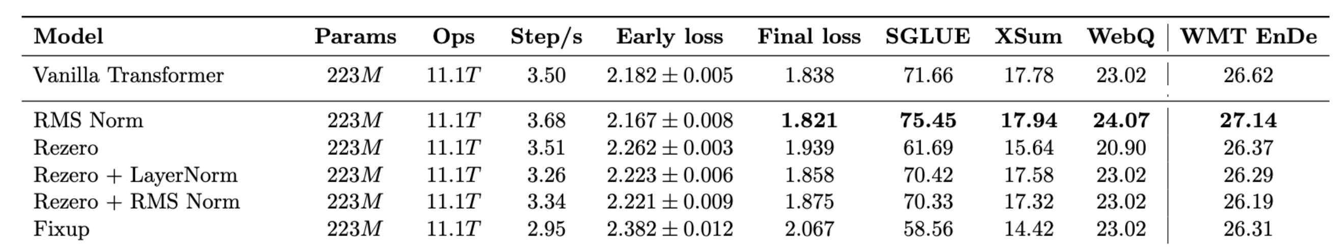
• Comparable performance: Practical evidence shows that RMSNorm is generally as effective as LayerNorm, and tabular data even indicates that RMSNorm shows slight improvements over Vanilla Transformer in Early Loss and Final Loss.

In fact, modern FFN structures have even dropped the bias term: \[ \underbrace{\text{FFN}(\boldsymbol{x}) = \max(0, \boldsymbol{x} \boldsymbol{W}_1 + \boldsymbol{b}_1) \boldsymbol{W}_2 + \boldsymbol{b}_2}_{\text{Original Transformer (ReLU, with bias term)}} \quad \longrightarrow \quad \underbrace{\text{FFN}(\boldsymbol{x}) = \sigma(\boldsymbol{x} \boldsymbol{W}_1) \boldsymbol{W}_2}_{\text{Modern Simplification (}\sigma\text{, without bias term)}} \]

Activation Functions

Activation functions are the core mechanism for introducing non-linearity in neural networks. In the Transformer architecture, the choice of activation function in FFN has evolved from ReLU to more complex gated mechanisms.

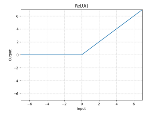
ReLU (Rectified Linear Unit)

\[ \text{FFN}(\boldsymbol{x}) = \max(0, \boldsymbol{x} \boldsymbol{W}_1) \boldsymbol{W}_2 \]

Low computational cost; outputs 0 when \(x \le 0\).

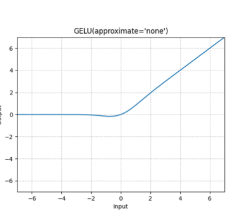
GeLU (Gaussian Error Linear Unit)

GeLU is a smooth activation function that introduces statistical concepts based on ReLU. \[ \text{FFN}(\boldsymbol{x}) = \text{GeLU}(\boldsymbol{x} \boldsymbol{W}_1) \boldsymbol{W}_2 \]

\[ \text{GeLU}(\boldsymbol{x}) = \boldsymbol{x} \cdot \Phi(\boldsymbol{x}) \]

Core concept: \(\Phi(\boldsymbol{x})\) is the cumulative distribution function (CDF).

\(\Phi(\boldsymbol{x})\) specifically refers to the CDF of the standard normal distribution.

• Definition of CDF: For a random variable \(X\), its CDF \(\boldsymbol{F}(\boldsymbol{x})\) is defined as \(P(X \le \boldsymbol{x})\), which is the probability that the random variable takes a value less than or equal to \(\boldsymbol{x}\). The range of CDF is always between \([0, 1]\).
• Role of \(\Phi(\boldsymbol{x})\): In GeLU, \(\Phi(\boldsymbol{x})\) acts as a smooth “gate” or weight factor:
  • When \(\boldsymbol{x}\) is a large positive number, \(\Phi(\boldsymbol{x}) \approx 1\) (the signal is fully retained).
  • When \(\boldsymbol{x}\) is negative, \(\Phi(\boldsymbol{x})\) gradually approaches \(0\) (the signal is smoothly suppressed).
• Graphical advantage: This multiplication operation based on CDF eliminates the non-differentiable sharp point of ReLU at \(\boldsymbol{x}=0\), making GeLU smooth everywhere, thus improving training stability in deep networks.

GLU (Gated Linear Unit)

The GLU family introduces a more complex gating mechanism and is considered one of the most powerful FFN activation mechanisms currently.

GLU is the foundation of all gated activations; it not only performs a simple non-linear transformation on the input but also uses two independent linear projections to control the flow of information.

• Core structure: Compared to \(\text{FF}(\boldsymbol{x}) = \max(0, \boldsymbol{x}\boldsymbol{W}_1)\boldsymbol{W}_2\): GLU introduces an additional parameter matrix \(\boldsymbol{V}\). It replaces \(\max(0, \boldsymbol{x}\boldsymbol{W}_1)\) with \(\max(0, \boldsymbol{x}\boldsymbol{W}_1) \otimes (\boldsymbol{x}\boldsymbol{V})\) (ReGLU).
• Gating mechanism: (\(\boldsymbol{x}\boldsymbol{V}\)) serves as the gating signal, controlling the amount of information flow through the activation function via element-wise multiplication (\(\otimes\)).
• Advantage: Enhances the model’s non-linear expressiveness, proven to yield consistent performance gains.

GeGLU (Gated GeLU)

• Formula: \(\text{FFN}_{\text{GeGLU}}(\boldsymbol{x}, \boldsymbol{W}, \boldsymbol{V}, \boldsymbol{W}_2) = (\text{GeLU}(\boldsymbol{x} \boldsymbol{W}) \otimes \boldsymbol{x} \boldsymbol{V}) \boldsymbol{W}_2\)

• Characteristics: Combines the smoothness of GeLU with the gating mechanism.

SwiGLU (Gated Swish)

• Formula: \(\text{FFN}_{\text{SwiGLU}}(\boldsymbol{x}, \boldsymbol{W}, \boldsymbol{V}, \boldsymbol{W}_2) = (\text{Swish}_1(\boldsymbol{x} \boldsymbol{W}) \otimes \boldsymbol{x} \boldsymbol{V}) \boldsymbol{W}_2\), where \(\text{Swish}(\boldsymbol{x}) = \boldsymbol{x} \cdot \text{sigmoid}(\boldsymbol{x})\).
• Status: Currently one of the most popular and powerful activation functions.

Swish function: \[ \text{Swish}(\boldsymbol{x}) = \boldsymbol{x} \cdot \text{sigmoid}(\boldsymbol{x}) \] where \(\text{sigmoid}(\boldsymbol{x}) = \frac{1}{1 + e^{-\boldsymbol{x}}}\).

The characteristics of the Swish activation function often make it superior to ReLU in practice:

• Smoothness: Swish is a smooth function that is differentiable everywhere. This is similar to GeLU, avoiding the sharp corner of ReLU at \(x=0\), which helps stabilize the optimization process.
• Non-monotonicity: Swish exhibits non-monotonicity on the negative half-axis (i.e., its curve decreases in the region where \(x < 0\), reaches a minimum, and then gradually approaches zero), allowing the model to retain or assign some weight to negative information, enhancing the model’s expressiveness.

Summary

The preferred activation functions for modern LLMs are SwiGLU or GeGLU, which introduce gating structures, simplify implementations by removing bias terms, and provide consistent performance gains, thereby enhancing the model’s expressiveness. However, it is still important to note that GLU is not the only necessary condition for building excellent models (e.g., GPT-3 still uses GeLU).

Serial vs. Parallel

The traditional serial computation method computes Attention and its residual connections first, then uses the Attention results as input for FFN, followed by computing FFN and its residual connections. In this case, Attention and FFN must wait for the previous computation to complete sequentially.

To improve training efficiency, some modern models, represented by GPT-J, PaLM, and GPT-NeoX, have introduced a parallel structure. The core idea is: Attention and FFN share the same input and compute simultaneously.

• Input Sharing: Both the Attention Block and MLP Block receive the original input \(\boldsymbol{x}\) after LayerNorm as their input signal.
• Parallel Computation: The two sub-layers compute their results independently and simultaneously.
• Residual Merging: The outputs of the two sub-layers (Attention gain and MLP gain) are combined back to the original input \(\boldsymbol{x}\) through a single residual connection, forming the final output \(\boldsymbol{y}\).

\[ \boldsymbol{y} = \boldsymbol{x} + \text{MLP}(\text{LayerNorm}(\boldsymbol{x})) + \text{Attention}(\text{LayerNorm}(\boldsymbol{x})) \]

The parallel structure is adopted mainly due to significant training acceleration:

• Speed Improvement: The parallel structure can achieve about 15% training speedup during large-scale training.
• Matrix Fusion: This acceleration primarily benefits from matrix multiplication fusion. Since the input matrix multiplications of Attention and MLP can be merged, it reduces memory access and computational overhead.
• Performance Assurance: Experiments have shown that if implemented properly, parallelization has minimal degradation on model quality, even negligible.

Embedding

Due to the permutation-invariant nature of the Transformer’s Self-Attention mechanism, we must explicitly inject positional information. The evolution of positional encoding in modern LLMs mainly revolves around “how to better capture relative positions.”

Sine Embeddings

\[ Embed(x, i) = v_x + PE_{pos} \\ PE_{(pos, 2i)} = \sin(pos/10000^{2i/d_{\text{model}}}) \\ PE_{(pos, 2i+1)} = \cos(pos/10000^{2i/d_{\text{model}}}) \]

Although it possesses the mathematical properties of relative positions, the expanded terms in the Attention computation \(\langle v_x + p_i, v_y + p_j \rangle\) will include messy cross-terms, such as \(\langle v_x, PE_j \rangle\). These terms mix content and positional information and are considered noise.

Absolute Embeddings

\[ Embed(x, i) = v_x + u_i \]

Directly learns a trainable vector for each position \(i\).

Limitations: Clearly not relative (obviously not relative), and has poor extrapolation capabilities, making it difficult to handle sequences longer than the training length.

Relative Embeddings

Directly adds a bias term \(a_{ij}\) in the Attention computation. The formula is \[ e_{ij} = \frac{x_i W^Q (x_j W^K + a_{ij}^K)^T}{\sqrt{d_z}} \] Although it solves the relative position problem, it is no longer in the standard inner product form (not an inner product), increasing the complexity of computational implementation.

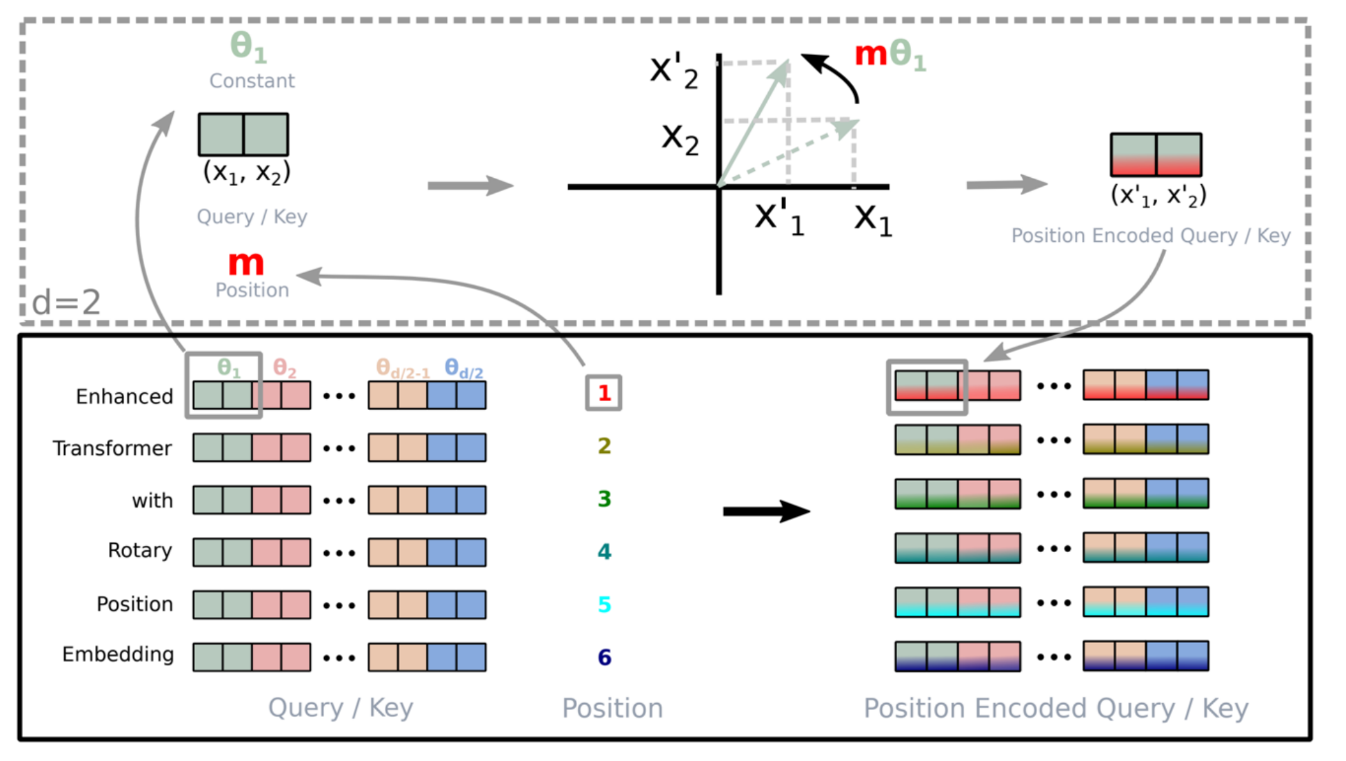
RoPE: Rotary Position Embeddings

RoPE is the standard configuration for current SOTA models (like LLaMA, PaLM, GPT-J). Its design aims to meet a core mathematical goal: High level thought process: to find a coding function \(f(x, i)\) such that the inner product of two vectors depends only on their relative distance \(i-j\). That is: \[ \langle f(x, i), f(y, j) \rangle = g(x, y, i - j) \] RoPE utilizes the property of vector inner products being invariant to rotation.

• Mechanism: RoPE does not perform at the Input Layer but rather applies rotation operations on \(Q\) and \(K\) at the Attention layer.
• Method: It splits vectors into pairs in a two-dimensional plane. For position \(m\), it rotates the vector by an angle of \(m\theta\) in the plane. Regardless of the absolute position, as long as the relative distance between two tokens is fixed, their rotated relative angle remains fixed, thus perfectly capturing relative positional information through the inner product.

image-20251216194036939

Hyperparameters & Dimensions

Attention Dimensions: The “1-1 Ratio”

In standard Transformer design, it is common to maintain Head_Dim \(\times\) Head_Num = Model_Dim (i.e., \(d_p \cdot h = d_{model}\)).

Low-Rank Bottleneck Controversy:

• Theoretical research [Bhojanapalli et al 2020] suggests that if Head_Dim (\(d_p\)) is too small, the rank of the Attention matrix will be limited, preventing the model from expressing certain complex attention patterns.
• The theory suggests: Head dimensions should be increased to break the 1-1 ratio.

Practical Conclusion: Experimental data (like Perplexity vs Parameters curves) shows that despite theoretical controversies, no significant low-rank bottleneck has been observed in practical engineering. Therefore, maintaining the standard 1-1 ratio remains the most efficient choice.

FFN Dimension Scaling (GLU Variant Scaling)

When using GLU variants like SwiGLU, due to the introduction of an additional gating matrix \(\boldsymbol{V}\) (increased parameter count), to keep the total parameter count consistent with the standard Transformer, the hidden layer dimension \(d_{ff}\) needs to be reduced.

Scaling Rule: Scale down by \(2/3\). \[ d_{ff} = \frac{8}{3} d_{model} \] This is why models like LLaMA typically have intermediate layer dimensions around 2.67 times \(d_{model}\), rather than the traditional 4 times.

Regularization

In training large-scale models, regularization strategies have shifted from “preventing overfitting” to “pursuing training efficiency and stability,” with the most significant change occurring in the use of Dropout.

Dropout

Dropout was once a standard regularization method in deep learning, preventing co-adaptation between neurons by randomly setting the outputs of neurons to zero during training, thus reducing overfitting.

Modern Trend (LLaMA / PaLM / Modern LLMs): Complete abandonment of Dropout (Dropout rate = 0). Current mainstream large models (like the LLaMA series, PaLM) typically do not use any Dropout during pre-training.

Reasons for Abandonment:

1. Data Scale: Modern LLMs are trained on trillions of tokens, often in an “underfitting” state rather than overfitting. The data itself serves as the best regularization.
2. Training Efficiency: Dropout requires storing random masks for backpropagation, increasing memory bandwidth overhead. In optimizations like FlashAttention, removing Dropout can significantly enhance computational throughput.
3. Training Stability: In extremely deep networks, the randomness introduced by Dropout can sometimes affect the stability of gradients.

Weight Decay

While Dropout has been discarded, Weight Decay remains an indispensable part of optimizers (like AdamW).

An additional penalty term is added to the loss function to suppress the norm of the weight matrix from becoming too large. It pulls the weight matrix back, avoiding overfitting. Essentially, we are telling the model: “Unless this feature is truly important, do not assign it such a large weight.” \[ \mathcal{L}_{total} = \mathcal{L}_{task} + \frac{\lambda}{2} \|\theta\|^2 \] General Setting: Typically set to \(0.1\) (as in GPT-3, LLaMA, PaLM).

Selective Application: Not all parameters use Weight Decay.

• Apply: Linear Layers (Attention projections, FFN weights).
• Skip: Bias terms, scaling factors \(\gamma\) of LayerNorm/RMSNorm, Embedding layers (sometimes). Applying Weight Decay to these parameters may disrupt numerical stability or the model’s adaptability to distributions.

Gradient Clipping

To prevent exploding gradients, this is a must-have in modern Transformer training.

• Mechanism: Monitor the \(L_2\) norm (\(|g|\)) of the global gradients. If it exceeds a threshold \(C\) (usually 1.0), scale the gradients: \[ \text{if } \|g\| > C, \quad g \leftarrow g \cdot \frac{C}{\|g\|} \]

• Effect: Even with RMSNorm and QK-Norm, during the initial training phase or when encountering “bad data,” Gradient Clipping remains the last line of defense to ensure training does not collapse.

Training Stability

Gradient Norm & Attention Optimizations

Phenomenon: Unoptimized models (like OLMo 0424) frequently exhibit severe gradient spikes during training, leading to significant loss curve spikes and potential divergence in training.

Optimization: By improving Attention computation (such as QK-Norm or Logit Softcapping), the gradient norm (L2 norm) can be kept very low and smooth, achieving an extremely stable training process.

QK-Norm (Query-Key Normalization)

In standard Attention computation, \(Q\) and \(K\) are multiplied directly: \[ \text{Score} = \frac{Q K^T}{\sqrt{d}} \] If the model allows the vector norms of \(Q\) or \(K\) to become very large during training, their inner product (dot product) will also become enormous. Even dividing by \(\sqrt{d}\) cannot offset this growth.

QK-Norm applies LayerNorm (or RMSNorm) to \(Q\) and \(K\) before performing matrix multiplication: \[ Q' = \text{LayerNorm}(Q) \\ K' = \text{LayerNorm}(K) \\ \text{Score} = \frac{Q' (K')^T}{\sqrt{d}} \] Why does it stabilize training?

1. Decoupling magnitude from direction: The essence of Attention is to compute the “similarity” (directional consistency) of vectors. QK-Norm forces the vectors to project onto a fixed hypersphere, eliminating interference from magnitude and allowing the model to focus on learning vector directions.
2. Preventing numerical explosion: Since LayerNorm restricts outputs within a specific statistical distribution (usually with variance 1), the result of \(Q \cdot K^T\) is naturally limited to a reasonable numerical range, avoiding logits values in the thousands or even tens of thousands.

Logit Softcapping

This is a key technique used in Gemma 2 and OLMo 2. Compared to QK-Norm’s input normalization, Logit Softcapping performs non-linear truncation on the output results. This, along with the z-loss discussed below, optimizes the stability of softmax.

It uses the \(\tanh\) function to limit logits within a fixed range (e.g., \([-C, C]\)). \[ \text{Logits}_{\text{capped}} = C \cdot \tanh\left(\frac{q^T k}{C \cdot \sqrt{d}}\right) \] where \(C\) is a hyperparameter (Cap value), typically set to 30 or 50.

Why does it stabilize training?

1. Hard Bound: The range of \(\tanh(x)\) is \((-1, 1)\). As \(x\) approaches 0, \(\tanh(u) \approx u\), maintaining linearity when the numbers are small, making this method almost ineffective at that point. However, when \(x\) is large, \(\tanh\) approaches 1 or -1, thus being limited within the \([-C, C]\) range. Therefore, regardless of how large \(q^T k\) is computed, the final logits’ absolute value will never exceed \(C\).
2. Preventing Softmax entropy collapse: If a logit value is extremely large (e.g., 1000), after applying softmax, the probability will become 1 (one-hot), while others become 0, leading to gradient vanishing. Softcapping ensures that the probability distribution output by softmax retains a certain level of entropy (uncertainty), allowing gradients to continue flowing back.

Output Softmax Stability: The “z-loss”

To address the numerical overflow issue of the output layer softmax (logits being too large leading to the partition function \(Z(x)\) exploding), PaLM introduced the z-loss trick.

Principle: An auxiliary penalty term is added to the total loss, encouraging the partition function \(\log Z\) to approach 0, at which point \(Z\) approaches 1. \[ Z(x) = \sum_{i} e^{z_i} \\ L_{\text{total}} = L_{\text{original}} + 10^{-4} \cdot \log^2 Z \] Application: This technique is primarily used for numerical stability during low-precision (bfloat16) training on TPU/GPU and has been widely adopted by models like Baichuan 2, DCLM, OLMo 2, etc.

Attention Efficiency

As the context window of models increases, memory usage and bandwidth during inference become major bottlenecks. Although the core architecture of the Transformer remains largely unchanged, significant adjustments have been made to the design of Attention Heads for efficiency.

Inference Bottleneck: Incremental Generation & KV Cache

During text generation, the model generates tokens step-by-step and cannot parallelize.

KV Cache: To avoid recalculating the Attention for all previous tokens each time a new token is generated, we must cache the Key and Value matrices of all previous tokens.

Memory Pressure: As the sequence lengthens, the size of the KV Cache grows linearly, potentially exceeding the memory usage of the model weights. This limits the maximum batch size and context length.

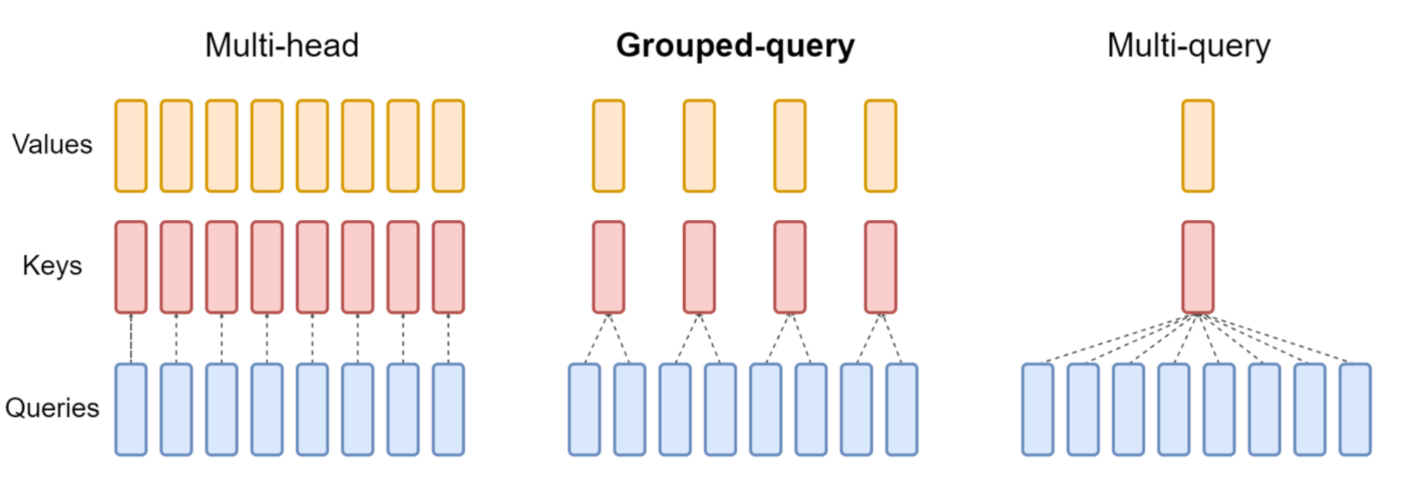
Optimization Solutions: GQA / MQA

To address the issue of oversized KV Cache, modern models reduce the number of Key/Value Heads to lower inference costs.

• MQA (Multi-Query Attention):
  • Mechanism: All Query Heads share the same Key Head and Value Head.
  • Advantage: Extreme memory savings and inference acceleration.
• GQA (Grouped Query Attention):
  • Mechanism: Groups Query Heads, with each group sharing a KV Head. For example, LLaMA 2/3.
  • Positioning: This is a compromise solution, balancing inference efficiency and model performance.

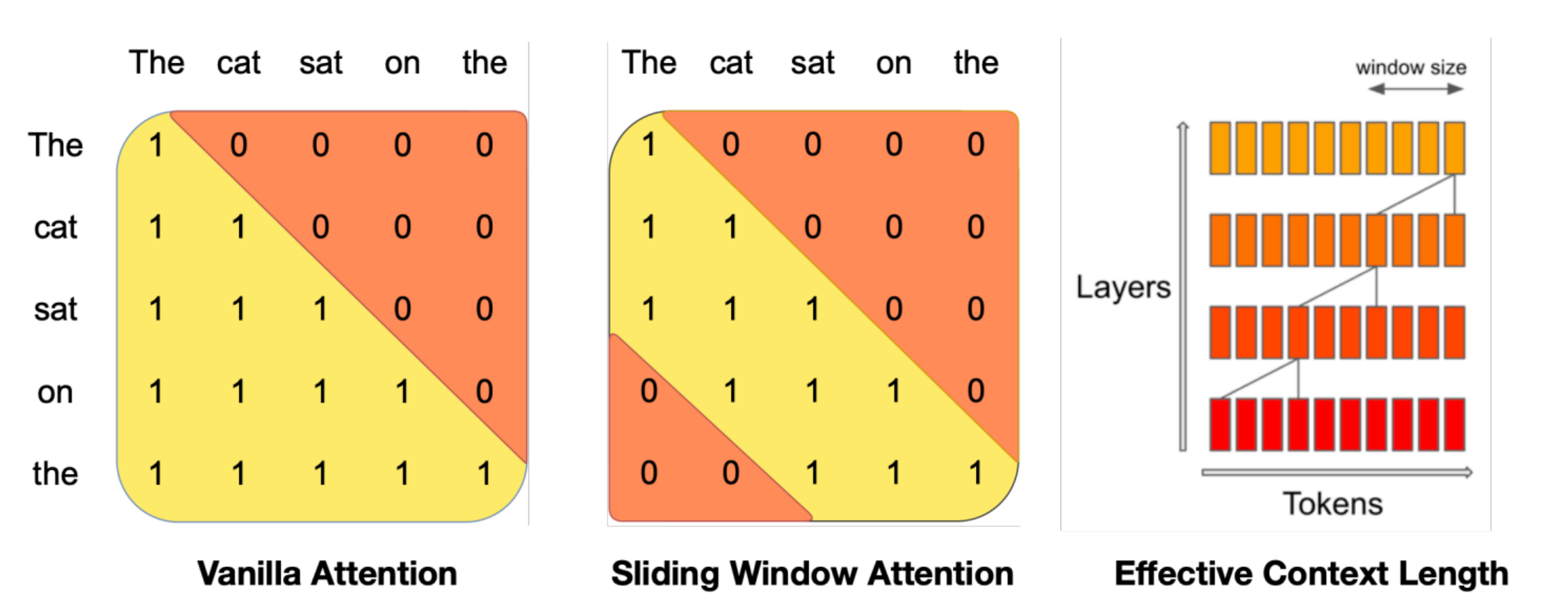
Other Attention Variants

Sparse / Sliding Window Attention: Models like Mistral and GPT-4 reduce complexity from \(O(N^2)\) by limiting Attention to only recent windows or sparse points, enabling them to handle extremely long texts.