Convolutional Neural Networks (CNN) - Part 1

Firstly, we know some facts about MLPs (Multi-Layer Perceptrons):

MLPs are universal function approximators. (Boolean functions, classifiers, and regressions)
MLPs can be trained through variations of gradient descent

But how do we meet the need of shift invariance, conventional MLPs are sensitive to the location of the pattern, resulting in a very large network to cover all possible locations of the pattern. So CNNs are introduced.

There are two scenarios in this lecture:

1D input (e.g., time series)
2D input (e.g., images)

Regular networks vs. Scanning networks

Regular networks

In a regular MLP, every neuron in the same layer is connnected by a unique weight to every unit in the previous layer.

All entries in the weight matrix are unique
The weight matrix is (generally) full

Scanning networks

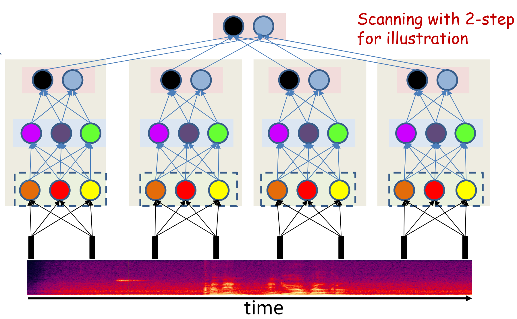
In a scanning MLP each neuron is connected to a subset of neurons in the previous layer.

The weight matrix is sparse
The weights matrix is block structured with identical blocks
The network is a shared parameter model

Scanning Networks are our focus in this lecture.

Learning in shared parameter model

Shared parameter model

1) Shared Parameters

Multiple connections are constrained to have the same parameter: \[ w_{ij}^k = w_{mn}^l = w^s \]

For any training instance $X$, a small perturbation of $w^s$ will simultaneously perturb both $w_{ij}^k$ and $w_{mn}^l$. Each of these perturbations will individually influence the final divergence (loss):
\[ Div(d, y) \]

The gradient with respect to the shared parameter $w^s$ equals the sum of the gradients with respect to each shared weight:
\[ \frac{\partial Div}{\partial w^s} = \frac{\partial Div}{\partial w_{ij}^k} \cdot \frac{\partial w_{ij}^k}{\partial w^s} + \frac{\partial Div}{\partial w_{mn}^l} \cdot \frac{\partial w_{mn}^l}{\partial w^s} \] Since $w_{ij}^k = w_{mn}^l = w^s$, this simplifies to:
\[ \frac{\partial Div}{\partial w^s} = \frac{\partial Div}{\partial w_{ij}^k} + \frac{\partial Div}{\partial w_{mn}^l} \] z In conclusion, the gradient with respect to a shared parameter is the sum of the gradients with respect to each of its instances.

2) Gradient of Shared Parameters

$S = \{e_1, e_2, ..., e_N\}$ is a set of shared edges. So the total gradient is the sum over all edges in the set:
\[ \frac{\partial Div}{\partial w^s} = \sum_{e \in S} \frac{\partial Div}{\partial w^e} \]

Then the loss gradient w.r.t. $w^s$ is \[ \nabla_S \mathrm{Loss} = \frac{\partial \mathrm{Loss}}{\partial w^s} = \sum_{e \in S} \frac{\partial \mathrm{Loss}}{\partial w^{e}}. \]

3) Gradient Descent Update

With learning rate $\eta$, update the shared parameter: \[ w^s \leftarrow w^s - \eta \ \nabla_S \mathrm{Loss}. \]

After updating, write the new shared value back to every tied weight: \[ \forall (k,i,j)\in S:\quad w^{(k)}_{i,j} \leftarrow w^s. \]

4) Training Loop

Initialize all weights $ _1, _2, , _K $.
For each tied set $S$:
- Backprop to get $ $ for each edge $e\in S$.
- Sum to obtain $ _S $.
- Update $ w^s w^s - , _S $.
- Sync the updated $ w^s $ back to all $ w^{(k)}_{i,j} S $.
Repeat until the loss converges.

Distributed vs Non-distributed Scanning

Definition

Distributed scanning: Parameters (weights) are shared across spatial positions.
→ Example: convolution kernels reused at every location.
Non-distributed scanning: Parameters are not shared; each location/block has its own set of weights.

Key Differences

Parameter sharing: Distributed ✅ | Non-distributed ❌
Parameter count:
- Distributed: Independent of number of positions; fewer parameters.
  - Formula: $K_0 D N_1 + K_1 N_1 N_2 + N_2 N_3$
- Non-distributed: Grows linearly with the number of positions (replicated per location).
Inductive bias:
- Distributed: Enforces translation equivariance/invariance.
- Non-distributed: No such bias; more flexible but prone to overfitting.
Output arrangement:
- Distributed: Naturally produces feature maps aligned with the input grid.
- Non-distributed: Not required to follow the same shape (can just collect outputs).
Efficiency:
- Distributed: Fewer parameters, better generalization, cheaper in memory/compute.
- Non-distributed: Many more parameters, expensive, less scalable.
Implementation analogy:
- Distributed ≈ Convolution (shared kernels).
- Non-distributed ≈ Independent MLPs applied at each location.

One-liner

The essence: Distributed vs non-distributed scanning differs in whether weights are shared across positions — which directly impacts parameter count, generalization, and efficiency.

Terminology in CNNs

Filter (Kernel): A learned weight tensor $W_c \in \mathbb{R}^{K_h \times K_w \times C_{\text{in}}}$ reused at every location; output at $(u,v,c)$: $y(u,v,c)=\sigma(\langle \text{patch}(u,v), W_c\rangle + b_c)$.

Receptive Field: The input region that affects a neuron’s output; per layer (1D) $r_l=r_{l-1}+(k_l-1)\,d_l\,j_{l-1}$, $j_l=j_{l-1}s_l$ with $r_0=1, j_0=1$.

Stride: The step size when sliding the filter over the input; larger strides reduce output size.

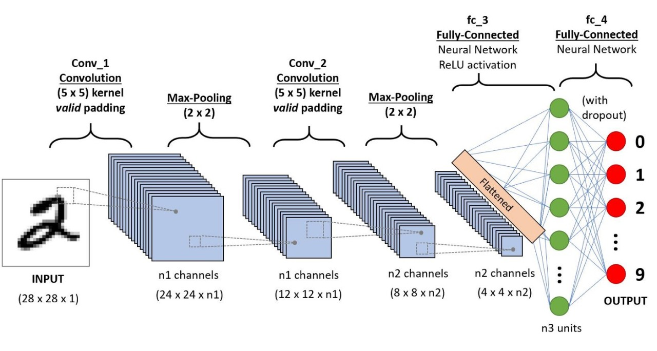
Flattening: reshape the final feature maps from shape $H \times W \times C$ into a 1-D vector of length $HWC$ (per sample) before feeding a fully connected/softmax layer.

With a classification head: train for classification by feeding the embedding $z$ into a linear layer + softmax (cross-entropy), predicting an ID among $C$ classes. Without a classification head: for verification, drop the linear/softmax and compare two embeddings $z_1,z_2$ with a similarity (e.g., cosine) to decide match vs non-match (threshold/EER).

Pooling: downsample local neighborhoods after conv;

max: $y=\max(x_1,\dots,x_K)$ keeps strongest response;
avg: $y=\tfrac{1}{K}\sum_{i=1}^K x_i$ smooths;

both reduce spatial size (stride $>1$) and add small shift/jitter invariance.

Summary

NN learn patterns hierarchically (simple → complex).
Pattern tasks = scan for target with a shared-parameter net (like CNN).
First layer scans input; higher layers scan previous maps; final layer makes decision.
Scanning can be distributed across layers; optional pooling adds small-shift invariance.
2-D scans → convnet; 1-D along time → TDNN.

CNNs - Part 1